2.6: Resonant Tunneling, and Metastable States

Now let us move to other, conceptually different quantum effects, taking place in more elaborate potential profiles. Neither piecewise-constant nor smooth-potential models of \(U(x)\) are convenient for their quantitative description because they both require "stitching" partial de Broglie waves at each classical turning point, which may lead to cumbersome calculations. However, we may get a very good insight of the physics of quantum effects that may take place in such profiles, using their approximation by sets of Dirac’s delta functions.

Additional help in studying such effects is provided by the notions of the scattering and transfer matrices, very useful for other cases as well. Consider an arbitrary but finite-length potential "bump" (formally called a scatterer), localized somewhere between points \(x_{1}\) and \(x_{2}\), on the flat potential background, say \(U=0\) (Fig. 12).

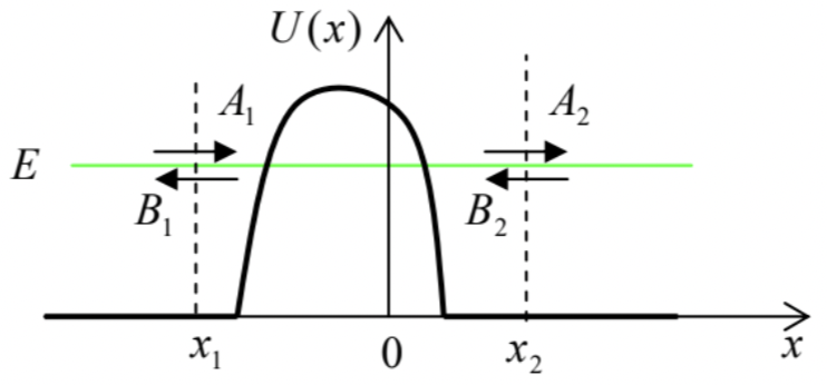Fig. 2.12. De Broglie wave amplitudes near a single 1D scatterer.

From Sec. 2, we know that the general solutions of the stationary Schrödinger equation, with a certain energy \(E\), outside the interval \(\left[x_{1}, x_{2}\right]\) are sets of two sinusoidal waves, traveling in the opposite directions. Let us represent them in the form \[\psi_{j}=A_{j} e^{i k\left(x-x_{j}\right)}+B_{j} e^{-i k\left(x-x_{j}\right)}\] where the index \(j\) (for now) is equal to either 1 or 2 , and \((\hbar k)^{2} / 2 m=E\). Note that each of the two wave pairs (129) has, in this notation, its own reference point \(x_{j}\), because this is very convenient for what follows. As we have already discussed, if the de Broigle wave/particle is incident from the left (i.e. \(B_{2}=\) \(0)\), the solution of the linear Schrödinger equation within the scatterer range \(\left(x_{1}<x<x_{2}\right)\) can provide only linear expressions for the transmitted \(\left(A_{2}\right)\) and reflected \(\left(B_{1}\right)\) wave amplitudes via the incident wave amplitude \(A_{1}\) : \[A_{2}=S_{21} A_{1}, \quad B_{1}=S_{11} A_{1},\] where \(S_{11}\) and \(S_{21}\) are certain (generally, complex) coefficients. Alternatively, if a wave, with amplitude \(B_{2}\), is incident on the scatterer from the right (i.e. if \(A_{1}=0\) ), it can induce a transmitted wave \(\left(B_{1}\right)\) and a reflected wave \(\left(A_{2}\right)\), with amplitudes \[B_{1}=S_{12} B_{2}, \quad A_{2}=S_{22} B_{2},\] where the coefficients \(S_{22}\) and \(S_{12}\) are generally different from \(S_{11}\) and \(S_{21}\). Now we can use the linear superposition principle to argue that if the waves \(A_{1}\) and \(B_{2}\) are simultaneously incident on the scatterer (say, because the wave \(B_{2}\) has been partly reflected back by some other scatterer located at \(x>x_{2}\) ), the resulting scattered wave amplitudes \(A_{2}\) and \(B_{1}\) are just the sums of their values for separate incident waves: \[\begin{aligned} &B_{1}=S_{11} A_{1}+S_{12} B_{2}, \\ &A_{2}=S_{21} A_{1}+S_{22} B_{2} . \end{aligned}\] These linear relations may be conveniently represented using the so-called scattering matrix \(\mathrm{S}\) : \[\left(\begin{array}{l} B_{1} \\ A_{2} \end{array}\right)=\mathrm{S}\left(\begin{array}{l} A_{1} \\ B_{2} \end{array}\right), \quad \text { with } \mathrm{S} \equiv\left(\begin{array}{ll} S_{11} & S_{12} \\ S_{21} & S_{22} \end{array}\right) .\] Scattering matrices, duly generalized, are an important tool for the analysis of wave scattering in more dimensions than one; for 1D problems, however, another matrix is often more convenient to represent the same linear relations (123). Indeed, let us solve this system for \(A_{2}\) and \(B_{2}\). The result is \[\begin{aligned} &A_{2}=T_{11} A_{1}+T_{12} B_{1}, \quad \text { i.e. }\left(\begin{array}{l} A_{2} \\ B_{2} \end{array}\right)=\mathrm{T}\left(\begin{array}{l} A_{1} \\ B_{1} \end{array}\right), \\ &B_{2}=T_{21} A_{1}+T_{22} B_{1}, \end{aligned}\] where \(\mathrm{T}\) is the transfer matrix, with the following elements: \[T_{11}=S_{21}-\frac{S_{11} S_{22}}{S_{12}}, \quad T_{12}=\frac{S_{22}}{S_{12}}, \quad T_{21}=-\frac{S_{11}}{S_{21}}, \quad T_{22}=\frac{1}{S_{12}} .\] The matrices \(S\) and \(T\) have some universal properties, valid for an arbitrary (but timeindependent) scatterer; they may be readily found from the probability current conservation and the time-reversal symmetry of the Schrödinger equation. Let me leave finding these relations for the reader’s exercise. The results show, in particular, that the scattering matrix may be rewritten in the following form: \[\mathrm{S}=e^{i \theta}\left(\begin{array}{cc} r e^{i \varphi} & t \\ t & -r e^{-i \varphi} \end{array}\right),\] where four real parameters \(r, t, \theta\), and \(\varphi\) satisfy the following universal relation: \[r^{2}+t^{2}=1,\] so that only 3 of these parameters are independent. As a result of this symmetry, \(T_{11}\) may be also represented in a simpler form, similar to \(T_{22}: T_{11}=\exp \{i \theta\} / t=1 / S_{12}{ }^{*}=1 / S_{21}{ }^{*}\). The last form allows a ready expression of the scatterer’s transparency via just one coefficient of the transfer matrix: \[\mathscr{T} \equiv\left|\frac{A_{2}}{A_{1}}\right|_{B_{2}=0}^{2}=\left|S_{21}\right|^{2}=\left|T_{11}\right|^{-2} .\] In our current context, the most important property of the 1D transfer matrices is that to find the total transfer matrix \(\mathrm{T}\) of a system consisting of several (say, \(N\) ) sequential arbitrary scatterers (Fig. 13), it is sufficient to multiply their matrices.

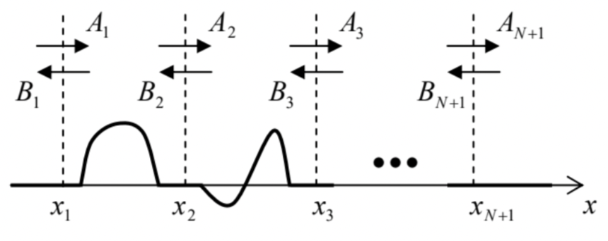Fig. 2.13. A sequence of several 1D scatterers.

Indeed, extending the definition (125) to other points \(x_{j}(j=1,2, \ldots, N+1)\), we can write \[\left(\begin{array}{l} A_{2} \\ B_{2} \end{array}\right)=\mathrm{T}_{1}\left(\begin{array}{l} A_{1} \\ B_{1} \end{array}\right), \quad\left(\begin{array}{l} A_{3} \\ B_{3} \end{array}\right)=\mathrm{T}_{2}\left(\begin{array}{l} A_{2} \\ B_{2} \end{array}\right)=\mathrm{T}_{2} \mathrm{~T}_{1}\left(\begin{array}{l} A_{1} \\ B_{1} \end{array}\right) \text {, etc. }\] (where the matrix indices correspond to the scatterers’ order on the \(x\)-axis), so that \[\left(\begin{array}{l} A_{N+1} \\ B_{N+1} \end{array}\right)=\mathrm{T}_{N} \mathrm{~T}_{N-1} \ldots \mathrm{T}_{1}\left(\begin{array}{l} A_{1} \\ B_{1} \end{array}\right) .\] But we can also define the total transfer matrix similarly to Eq. (125), i.e. as \[\left(\begin{array}{l} A_{N+1} \\ B_{N+1} \end{array}\right) \equiv \mathrm{T}\left(\begin{array}{l} A_{1} \\ B_{1} \end{array}\right),\] so that comparing Eqs. (130) and (131) we get \[\mathrm{T}=\mathrm{T}_{N} \mathrm{~T}_{N-1} \ldots \mathrm{T}_{1} .\] This formula is valid even if the flat-potential gaps between component scatterers are shrunk to zero, so that it may be applied to a scatterer with an arbitrary profile \(U(x)\), by fragmenting its length into many small segments \(\Delta x=x_{j+1}-x_{j}\), and treating each fragment as a rectangular barrier of the average height \(\left(U_{j}\right)_{\text {ef }}=\left[U\left(x_{j+1}\right)-U\left(x_{j}\right)\right] / 2-\) see Fig. 14. Since very efficient numerical algorithms are readily available for fast multiplication of matrices (especially as small as \(2 \times 2\) in our case), this approach is broadly used in practice for the computation of transparency of potential barriers with complicated profiles \(U(x)\). (Computationally, this procedure is much more efficient than the direct numerical solution of the stationary Schrödinger equation.)

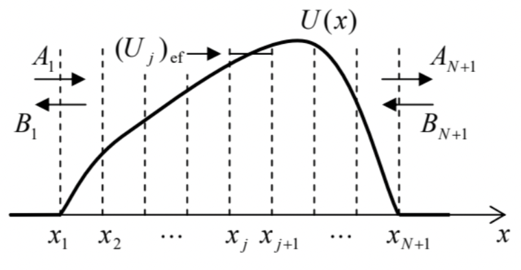Fig. 2.14. The transfer matrix approach to a potential barrier with an arbitrary profile.

In order to apply this approach to several particular, conceptually important systems, let us calculate the transfer matrices for a few elementary scatterers, starting from the delta-functional barrier located at \(x=0\) - see Fig. 8. Taking \(x_{1}, x_{2} \rightarrow 0\), we can merely change the notation of the wave amplitudes in Eq. (78) to get \[S_{11}=\frac{-i \alpha}{1+i \alpha}, \quad S_{21}=\frac{1}{1+i \alpha} .\] An absolutely similar analysis of the wave incidence from the left yields \[S_{22}=\frac{-i \alpha}{1+i \alpha}, \quad S_{12}=\frac{1}{1+i \alpha},\] and using Eqs. (126), we get \[\mathrm{T}_{\alpha}=\left(\begin{array}{cc} 1-i \alpha & -i \alpha \\ i \alpha & 1+i \alpha \end{array}\right) .\] As a sanity check, Eq. (128) applied to this result, immediately brings us back to Eq. (79).

The next example may seem strange at the first glance: what if there is no scatterer at all between the points \(x_{1}\) and \(x_{2}\) ? If the points coincide, the answer is indeed trivial and can be obtained, e.g., from Eq. (135) by taking \(w=0\), i.e. \(\alpha=0\) : \[\mathrm{T}_{0}=\left(\begin{array}{ll} 1 & 0 \\ 0 & 1 \end{array}\right) \equiv \mathrm{I}\]

• the so-called identity matrix. However, we are free to choose the reference points \(x_{1,2}\) participating in Eq. (120) as we wish. For example, what if \(x_{2}-x_{1}=a\) ? Let us first take the forward-propagating wave alone: \(B_{2}=0\) (and hence \(B_{1}=0\) ); then

\[\psi_{2}=\psi_{1}=A_{1} e^{i k\left(x-x_{1}\right)} \equiv A_{1} e^{i k\left(x_{2}-x_{1}\right)} e^{i k\left(x-x_{2}\right)} .\] The comparison of this expression with the definition (120) for \(j=2\) shows that \(A_{2}=A_{1} \exp \left\{i k\left(x_{2}-x_{1}\right)\right\}\) \(=A_{1} \exp \{i k a\}\), i.e. \(T_{11}=\exp \{i k a\}\). Repeating the calculation for the back-propagating wave, we see that \(T_{22}=\exp \{-i k a\}\), and since the space interval provides no particle reflection, we finally get \[\mathrm{T}_{a}=\left(\begin{array}{cc} e^{i k a} & 0 \\ 0 & e^{-i k a} \end{array}\right),\] independently of a common shift of points \(x_{1}\) and \(x_{2}\). At \(a=0\), we naturally recover the special case (136). Now let us use these simple results to analyze the double-barrier system shown in Fig. 15. We could of course calculate its properties as before, writing down explicit expressions for all five traveling waves shown by arrows in Fig. 15, then using the boundary conditions (124) and (125) at each of points \(x_{1,2}\) to get a system of four linear equations, and finally, solving it for four amplitude ratios.

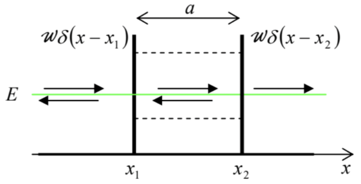Fig. 2.15. The double-barrier system. The dashed lines show (schematically) the quasilevels of the metastable-state energies.

However, the transfer matrix approach simplifies the calculations, because we may immediately use Eqs. (132), (135), and (138) to write \[\mathrm{T}=\mathrm{T}_{\alpha} \mathrm{T}_{a} \mathrm{~T}_{\alpha}=\left(\begin{array}{cc} 1-i \alpha & -i \alpha \\ i \alpha & 1+i \alpha \end{array}\right)\left(\begin{array}{cc} e^{i k a} & 0 \\ 0 & e^{-i k a} \end{array}\right)\left(\begin{array}{cc} 1-i \alpha & -i \alpha \\ i \alpha & 1+i \alpha \end{array}\right) .\] Let me hope that the reader remembers the "row by column" rule of the multiplication of square matrices \(;{ }^{27}\) using it for the last two matrices, we may reduce Eq. (139) to \[\mathrm{T}=\left(\begin{array}{cc} 1-i \alpha & -i \alpha \\ i \alpha & 1+i \alpha \end{array}\right)\left(\begin{array}{cc} (1-i \alpha) e^{i k a} & -i \alpha e^{i k a} \\ i \alpha e^{-i k a} & (1+i \alpha) e^{-i k a} \end{array}\right) .\] Now there is no need to calculate all elements of the full product \(\mathrm{T}\), because, according to Eq. (128), for the calculation of barrier’s transparency \(T\) we need only one its element, \(T_{11}\) : \[\mathscr{T}=\frac{1}{\left|T_{11}\right|^{2}}=\frac{1}{\left|\alpha^{2} e^{-i k a}+(1-i \alpha)^{2} e^{i k a}\right|^{2}} .\] This result is somewhat similar to that following from Eq. (71) for \(E>U_{0}\) : the transparency is a \(\pi\)-periodic function of the product \(k a\), reaching its maximum \((\mathscr{T}=1)\) at some point of each period - see Fig. 16a. However, Eq. (141) is different in that for \(\alpha>>1\), the resonance peaks of the transparency are very narrow, reaching their maxima at \(k a \approx k_{n} a \equiv n \pi\), with \(n=1,2, \ldots\)

The physics of this resonant tunneling effect \({ }^{28}\) is the so-called constructive interference, absolutely similar to that of electromagnetic waves (for example, light) in a Fabry-Perot resonator formed by two parallel semi-transparent mirrors. \({ }^{29}\) Namely, the incident de Broglie wave may either tunnel through the two barriers or undertake, on its way, several sequential reflections from these semitransparent walls. At \(k=k_{n}\), i.e. at \(2 k a=2 k_{n} a=2 \pi n\), the phase differences between all these partial waves are multiples of \(2 \pi\), so that they add up in phase - "constructively". Note that the same constructive interference of numerous reflections from the walls may be used to interpret the standingwave eigenfunctions (1.84), so that the resonant tunneling at \(\alpha \gg>1\) may be also considered as a result of the incident wave’s resonance induction of such a standing wave, with a very large amplitude, in the space between the barriers, with the transmitted wave’s amplitude proportionately increased.

Fig. 2.16. Resonant tunneling through a potential well with delta-functional walls: (a) the system’s transparency as a function of \(k a\), and (b) calculating the resonance’s FWHM at \(\alpha>>1\).

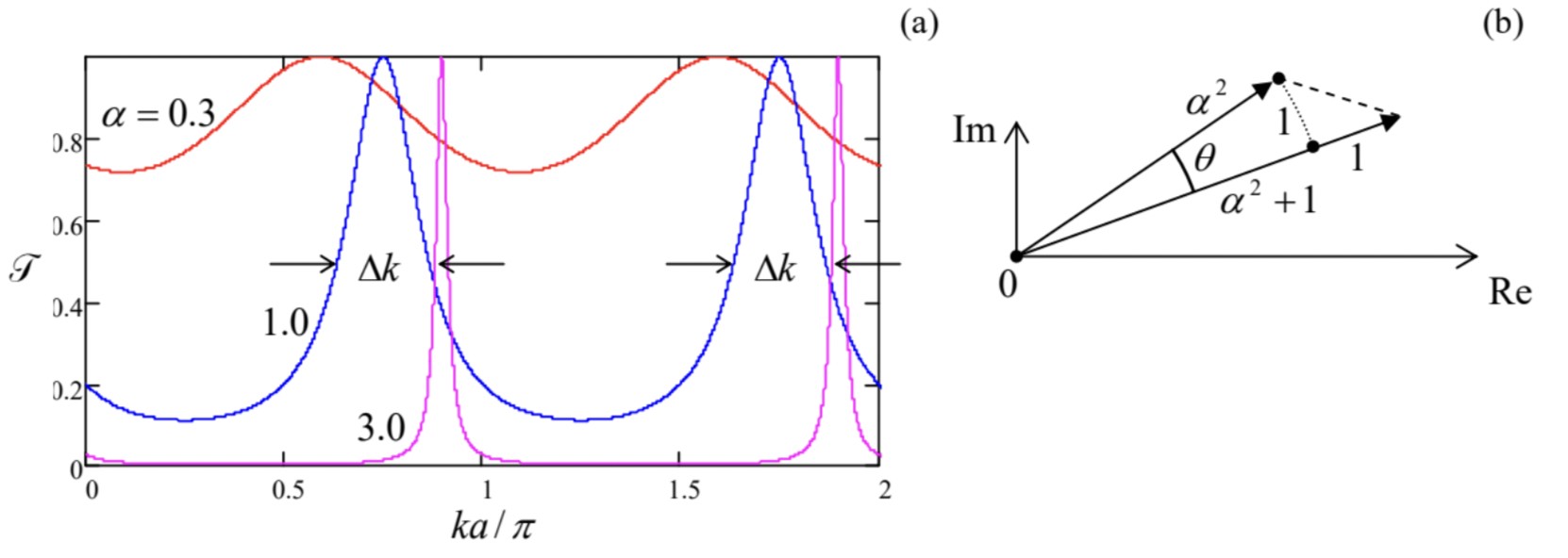
As a result of this resonance, the maximum transparency of the system is \(\operatorname{perfect}\left(\mathscr{T}_{\max }=1\right)\) even at \(\alpha \rightarrow \infty\), i.e. in the case of very low transparency of each of the two component barriers. Indeed, the denominator in Eq. (141) may be interpreted as the squared length of the difference between two 2D vectors, one of length \(\alpha^{2}\), and another of length \(\left|(1-i \alpha)^{2}\right|=1+\alpha^{2}\), with the angle \(\theta=2 k a+\) const between them - see Fig. 16b. At the resonance, the vectors are aligned, and their difference is smallest (equal to 1) so that \(\mathscr{T}_{\max }=1\). (This result is exact only if the two barriers are exactly equal.)

The same vector diagram may be used to calculate the so-called FWHM, a common acronym for the Full Width [of the resonance curve at its] Half-Maximum. By definition, this is the difference \(\Delta k=k_{+}\) \(-k\). between such two values of \(k\), on the opposite slopes of the same resonance, at that \(\mathscr{T}=\mathscr{T}_{\max } / 2-\operatorname{see}\) the arrows in Fig. 16a. Let the vectors in Fig. 16b, drawn for \(\alpha \gg>1\), be misaligned by a small angle \(\theta\) \(\sim 1 / \alpha^{2}<<1\), so that the length of the difference vector is much smaller than the length of each vector. To double its length squared, and hence to reduce \(\mathscr{T}\) by a factor of two in comparison with its maximum value 1 , the arc between the vectors, equal to \(\alpha^{2} \theta\), should also become equal to \(\pm 1\), i.e. \(\alpha^{2}\left(2 k_{\pm} a+\right.\) const \()\) \(=\pm 1\). Subtracting these two equalities from each other, we get \[\Delta k \equiv k_{+}-k_{-}=\frac{1}{a \alpha^{2}}<<k_{\pm} .\] Now let us use the simple system shown in Fig. 15 to discuss an issue of large conceptual significance. For that, consider what would happen if at some initial moment (say, \(t=0\) ) we have placed a 1D quantum particle inside the double-barrier well with \(\alpha \gg>1\), and left it there alone, without any incident wave. To simplify the analysis, let us assume that the initial state of the particle coincides with one of the stationary states of the infinite-wall well of the same size - see Eq. (1.84): \[\Psi(x, 0)=\psi_{n}(x)=\left(\frac{2}{a}\right)^{1 / 2} \sin \left[k_{n}\left(x-x_{1}\right)\right], \quad \text { where } k_{n}=\frac{\pi n}{a}, \quad n=1,2, \ldots .\] At \(\alpha \rightarrow \infty\), this is just an eigenstate of the system, and from our analysis in Sec. \(1.5\) we know the time evolution of its wavefunction: \[\Psi(x, t)=\psi_{n}(x) \exp \left\{-i \omega_{n} t\right\}=\left(\frac{2}{a}\right)^{1 / 2} \sin \left[k_{n}\left(x-x_{1}\right)\right] \exp \left\{-i \omega_{n} t\right\}, \quad \text { with } \omega_{n}=\frac{E_{n}}{\hbar}=\frac{\hbar k_{n}^{2}}{2 m},\] telling us that the particle remains in the well at all times with constant probability \(W(t)=W(0)=1\).

However, if the parameter \(\alpha\) is large but finite, the de Broglie wave would slowly "leak out" from the well, so that \(W(t)\) would slowly decrease. Such a state is called metastable. Let us derive the law of its time evolution, assuming that at the slow leakage, with a characteristic time \(\tau \gg 1 / \omega_{n}\), does not affect the instant wave distribution inside the well, besides the gradual, slow reduction of \(W .^{30}\) Then we can generalize Eq. (144) as \[\Psi(x, t)=\left(\frac{2 W}{a}\right)^{1 / 2} \sin \left[k_{n}\left(x-x_{1}\right)\right] \exp \left\{-i \omega_{n} t\right\} \equiv A \exp \left\{i\left(k_{n} x-\omega_{n} t\right)\right\}+B\left\{-i\left(k_{n} x+\omega_{n} t\right)\right\},\] making the probability of finding the particle in the well equal to \(W \leq 1\). As the last form of Eq. (145) shows, this function is the sum of two traveling waves, with equal magnitudes of their amplitudes and equal but opposite probability currents (5): \[|A|=|B|=\left(\frac{W}{2 a}\right)^{1 / 2}, \quad I_{A}=\frac{\hbar}{m}|A|^{2} k_{n}=\frac{\hbar}{m} \frac{W}{2 a} \frac{\pi n}{a}, \quad I_{B}=-I_{A} .\] But we already know from Eq. (79) that at \(\alpha \gg>1\), the delta-functional wall’s transparency \(\mathscr{T}\) equals \(1 / \alpha^{2}\), so that the wave carrying current \(I_{A}\), incident on the right wall from the inside, induces an outcoming wave outside of the well (Fig. 17) with the following probability current:

Fig. 2.17. Metastable state’s decay in the simple model of a 1D potential well formed by two low-transparent walls – schematically.

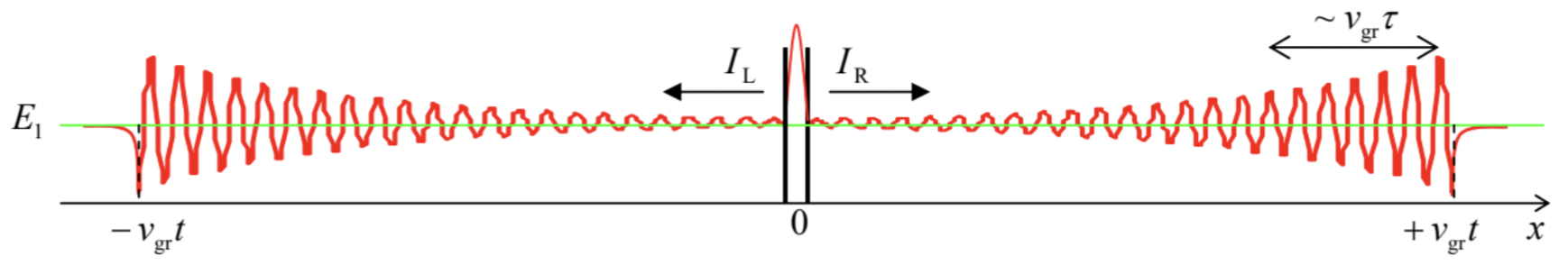
Fig. 2.17. Metastable state’s decay in the simple model of a 1D potential well formed by two low-transparent walls - schematically.

Absolutely similarly, \[I_{\mathrm{L}}=\frac{1}{\alpha^{2}} I_{B}=-I_{\mathrm{R}} .\] Now we may combine the 1D version (6) of the probability conservation law for the well’s interior: \[\frac{d W}{d t}+I_{\mathrm{R}}-I_{\mathrm{L}}=0,\] with Eqs. (147)-(148) to write \[\frac{d W}{d t}=-\frac{1}{\alpha^{2}} \frac{\pi n \hbar}{m a^{2}} W .\] This is just the standard differential equation, \[\frac{d W}{d t}=-\frac{1}{\tau} W,\] of the exponential decay, \(W(t)=W(0) \exp \{-t / \tau\}\), where the constant \(\tau\), in our case equal to \[\tau=\frac{m a^{2}}{\pi n \hbar} \alpha^{2},\] is called the metastable state’s lifetime. Using Eq. (2.33b) for the de Broglie waves’ group velocity, for our particular wave vector giving \(v_{\mathrm{gr}}=\hbar k_{n} / m=\pi n \hbar / m a\), Eq. (152) may be rewritten in a more general form, \[\tau=\frac{t_{\mathrm{a}}}{\mathscr{T}},\] where the attempt time \(t_{\mathrm{a}}\) is equal to \(a / v_{\mathrm{gr}}\), and (in our particular case) \(\mathcal{T}=1 / \alpha^{2}\), in which it is valid for a broad class of similar metastable systems. \({ }^{31}\) Equality may be interpreted in the following semi-classical way. The particle travels back and forth between the confining potential barriers, with the time interval \(t_{\mathrm{a}}\) between the sequential moments of incidence, each time attempting to leak through the wall, with the success probability equal to \(\mathscr{T}\), so the reduction of \(W\) per each incidence is \(\Delta W=-W \mathscr{T}\), in the limit \(\alpha \gg\) 1 (i.e. \(\mathscr{T}<<1\) ) immediately leading to the decay equation \((151)\) with the lifetime \((153)\).Another useful look at Eq. (152) may be taken by returning to the resonant tunneling problem in the same system, and expressing the resonance width (142) in terms of the incident particle’s energy: \[\Delta E=\Delta\left(\frac{\hbar^{2} k^{2}}{2 m}\right) \approx \frac{\hbar^{2} k_{n}}{m} \Delta k=\frac{\hbar^{2} k_{n}}{m} \frac{1}{a \alpha^{2}}=\frac{\pi n \hbar^{2}}{m a^{2} \alpha^{2}} .\] Comparing Eqs. (152) and (154), we get a remarkably simple, parameter-independent formula \(^{32}\) \[\Delta E \cdot \tau=\hbar\] This energy-time uncertainty relation is certainly more general than our simple model; for example, it is valid for the lifetime and resonance tunneling width of any metastable state in the potential profile of any shape. This seems very natural, since because of the energy identification with frequency, \(E=\hbar \omega\), typical for quantum mechanics, Eq. (155) may be rewritten as \(\Delta \omega \cdot \tau=1\) and seems to follow directly from the Fourier transform in time, just as the Heisenberg’s uncertainty relation (1.35) follows from the Fourier transform in space. In some cases, these two relations are indeed interchangeable; for example, Eq. (24) for the Gaussian wave packet width may be rewritten as \(\delta E \cdot \Delta t=\) \(\hbar\), where \(\delta E=\hbar(d \omega / d k) \delta k=\hbar v_{\mathrm{gr}} \delta k\) is the r.m.s. spread of energies of monochromatic components of the packet, while \(\Delta t \equiv \delta x / v_{\mathrm{gr}}\) is the time scale of packet’s passage through a fixed observation point \(x\).

However, Eq. (155) it is much less general than Heisenberg’s uncertainty relation (1.35). Indeed, in the non-relativistic quantum mechanics we are studying now, the Cartesian coordinates of a particle, the Cartesian components of its momentum, and the energy \(E\) are regular observables, represented by operators. In contrast, time is treated as a \(c\)-number argument, and is not represented by an operator, so that Eq. (155) cannot be derived in such general assumptions as Eq. (1.35). Thus the time-energy uncertainty relation should be used with caution. Unfortunately, not everybody is so careful. One can find, for example, wrong claims that due to this relation, the energy dissipated by any system performing an elementary (single-bit) calculation during a time interval \(\Delta t\) has to be larger than \(\hbar / \Delta t .{ }^{33}\) Another incorrect statement is that the energy of a system cannot be measured, during a time interval \(\Delta t\), with an accuracy better than \(\hbar / \Delta t .{ }^{34}\)

Now that we have a quantitative mathematical description of the metastable state’s decay (valid, again, only if \(\alpha \gg>1\), i.e. if \(\tau \gg t_{\mathrm{a}}\) ), we may use it for discussion of two important conceptual issues of quantum mechanics. First, this is one of the simplest examples of systems that may be considered, from two different points of view, as either Hamiltonian (and hence time-reversible), or open (and hence irreversible). Indeed, from the former point of view, our particular system is certainly described by a time-independent Hamiltonian of the type (1.41), with the potential energy \[U(x)=w\left[\delta\left(x-x_{1}\right)+\delta\left(x-x_{2}\right)\right]\]

• see Fig. 15 again. In this point of view, the total probability of finding the particle somewhere on the axis \(x\) remains equal to 1 , and the full system’s energy, calculated from Eq. (1.23),

\[\langle E\rangle=\int_{-\infty}^{+\infty} \Psi^{*}(x, t) \hat{H} \Psi(x, t) d^{3} x,\] remains constant and completely definite \((\delta E=0)\). On the other hand, since the "emitted" wave packets would never return to the potential well, \({ }^{35}\) it makes sense to look at the well’s region alone. For such a truncated, open system (for which the space beyond the interval \(\left[x_{1}, x_{2}\right]\) serves as its environment), the probability \(W\) of finding the particle inside this interval, and hence its energy \(\langle E\rangle=W E_{n}\), decay exponentially per Eq. (151) - the decay equation typical for irreversible systems. We will return to the discussion of the dynamics of such open quantum systems in Chapter \(7 .\)

Second, the same model enables a preliminary discussion of one important aspect of quantum measurements. As Eq. (151) and Fig. 17 show, at \(t \gg \tau\), the well becomes virtually empty \((W \approx 0)\), and the whole probability is localized in two clearly separated wave packets with equal amplitudes, moving from each other with the speed \(v_{\mathrm{gr}}\), each "carrying the particle away" with a probability of \(50 \%\). Now assume that an experiment has detected the particle on the left side of the well. Though the formalisms suitable for quantitative analysis of the detection process will not be discussed until Chapter 7 , due to the wide separation \(\Delta x=2 v_{\mathrm{gr}} t>>2 v_{\mathrm{gr}} \tau\) of the packets, we may safely assume that such detection may be done without any actual physical effect on the counterpart wave packet. \({ }^{36}\) But if we know that the particle has been found on the left side, there is no chance to find it on the right side. If we attributed the full wavefunction to all stages of this particular experiment, this situation might be rather confusing. Indeed, that would mean that the wavefunction at the right packet’s location should instantly turn into zero - the so-called wave packet reduction (or "collapse") - a hypothetical, irreversible process that cannot be described by the Schrödinger equation for this system, even including the particle detectors.

However, if (as was already discussed in Sec. 1.3) we attribute the wavefunction to a certain statistical ensemble of similar experiments, there is no need to involve such an artificial notion. The two-packet picture we have calculated (Fig. 17) describes the full ensemble of experiments with all systems prepared in the initial state (143), i.e. does not depend on the particle detection results. On the other hand, the "reduced packet" picture (with no wave packet on the right of the well) describes only a sub-ensemble of such experiments, in which the particles have been detected on the left side. As was discussed on classical examples in Sec. 1.3, for such redefined ensemble the probability distribution is rather different. So, the "wave packet reduction" is just a result of a purely accounting decision of the observer. \({ }^{37}\) I will return to this important discussion in Sec. \(10.1\) - on the basis of the forthcoming discussion of open systems in Chapters 7 and 8 .

---

\({ }^{27}\) In an analytical form: \((\mathrm{AB})_{j j^{\prime}}=\sum_{j^{\prime \prime}=1}^{N} A_{i j^{\prime \prime}} B_{j^{\prime \prime \prime}}\), where \(N\) is the matrix rank (in our current case, \(N=2\) ).

\({ }^{28}\) In older literature, it is sometimes called the Townsend (or "Ramsauer-Townsend") effect. However, it is more common to use that term only for a similar effect at 3D scattering - to be discussed in Chapter \(3 .\)

\({ }^{29}\) See, e.g., EM Sec. \(7.9\).

\({ }^{30}\) This virtually evident assumption finds its formal justification in the perturbation theory to be discussed in Chapter 6.

\({ }^{31}\) Essentially the only requirement is to have the attempt time \(\Delta t_{\mathrm{A}}\) to be much longer than the effective time (the instanton time, see Sec. \(5.3\) below) of tunneling through the barrier. In the delta-functional approximation for the barrier, the latter time is equal to zero, so that this requirement is always fulfilled.

\({ }^{32}\) Note that the metastable state’s decay (2.151) may be formally obtained from the basic Schrödinger equation (1.61) by adding an imaginary part, equal to \((-\Delta E / 2)\), to its eigenenergy \(E_{n}\). Indeed, in this case Eq. (1.62) becomes \(a_{n}(t)=\) const \(\times \exp \left\{-i\left(E_{n}-i \Delta E / 2\right\} t / \hbar\right\} \equiv\) const \(\times \exp \left\{-i E_{n} t / \hbar\right\} \times \exp \{-\Delta E t / 2 \hbar\}=\) const \(\times \exp \left\{-i E_{n} t / \hbar\right\} \times \exp \{-\) \(t / 2 \tau\}\), so that \(W(t) \propto\left|a_{n}(t)\right|^{2} \propto \exp \{-t / \tau\}\). Such formalism, which hides the physical origin of the state’s decay, may be convenient for some calculations, but misleading in other cases, and I will not use it in this course.

\({ }^{33}\) On this issue, I dare to refer the reader to my own old work K. Likharev, Int. J. Theor. Phys. 21,311 (1982), which provided a constructive proof (for a particular system) that at reversible computation, whose idea had been put forward in 1973 by C. Bennett (see, e.g., SM Sec. 2.3), energy dissipation may be lower than this apparent "quantum limit".

\({ }^{34}\) See, e.g., a discussion of this issue in the monograph by V. Braginsky and F. Khalili, Quantum Measurement, Cambridge U. Press, 1992 .

\({ }^{35}\) For more realistic 2D and 3D systems, this statement is true even if the system as a whole is confined inside some closed volume, much larger than the potential well housing the metastable states. Indeed, if the walls

\({ }^{36}\) This argument is especially convincing if the particle’s detection time is much shorter than the time \(t_{c}=2 v_{\mathrm{gr}} t / c\), where \(c\) is the speed of light in vacuum, i.e. the maximum velocity of any information transfer.

\({ }^{37}\) "The collapse of the wavefunction after measurement represents nothing more than the updating of that scientist’s expectations." N. D. Mermin, Phys. Today, 72, 53 (Jan. 2013).