2.5: Motion in Soft Potentials

Before moving on to exploring other quantum-mechanical effects, let us see how the results discussed in the previous section are modified in the opposite limit of the so-called soft (also called "smooth") potential profiles, like the one sketched in Fig. \(3 .{ }^{19}\) The most efficient analytical tool to study this limit is the so-called WKB (or "JWKB", or "quasiclassical") approximation developed by H. Jeffrey, G. Wentzel, A. Kramers, and L. Brillouin in 1925-27. In order to derive its 1D version, let us rewrite the Schrödinger equation (53) in a simpler form \[\frac{d^{2} \psi}{d x^{2}}+k^{2}(x) \psi=0,\] where the local wave number \(k(x)\) is defined similarly to Eq. (65), \[k^{2}(x) \equiv \frac{2 m[E-U(x)]}{\hbar^{2}}\] besides that now it may be a function of \(x\). We already know that for \(k(x)=\) const, the fundamental solutions of this equation are \(A \exp \{+i k x\}\) and \(B \exp \{-i k x\}\), which may be represented in a single form \[\psi(x)=e^{i \Phi(x)},\] where \(\Phi(x)\) is a complex function, in these two simplest cases being equal, respectively, to \((k x-i \ln A)\) and \((-k x-i \ln B)\). This is why we may try use Eq. (83) to look for solution of Eq. (81) even in the general case, \(k(x) \neq\) const. Differentiating Eq. (83) twice, we get \[\frac{d \psi}{d x}=i \frac{d \Phi}{d x} e^{i \Phi}, \quad \frac{d^{2} \psi}{d x^{2}}=\left[i \frac{d^{2} \Phi}{d x^{2}}-\left(\frac{d \Phi}{d x}\right)^{2}\right] e^{i \Phi} .\] Plugging the last expression into Eq. (81) and requiring the factor before \(\exp \{i \Phi(x)\}\) to vanish, we get \[i \frac{d^{2} \Phi}{d x^{2}}-\left(\frac{d \Phi}{d x}\right)^{2}+k^{2}(x)=0 .\] This is still an exact, general equation. At the first sight, it looks harder to solve than the initial equation (81), because Eq. (85) is nonlinear. However, it is ready for simplification in the limit when the potential profile is very soft, \(d U / d x \rightarrow 0\). Indeed, for a uniform potential, \(d^{2} \Phi / d x^{2}=0\). Hence, in the socalled \(0^{\text {th }}\) approximation, \(\Phi(x) \rightarrow \Phi_{0}(x)\), we may try to keep that result, so that Eq. (85) is reduced to \[\left(\frac{d \Phi_{0}}{d x}\right)^{2}=k^{2}(x), \quad \text { i.e. } \frac{d \Phi_{0}}{d x}=\pm k(x), \quad \Phi_{0}(x)=\pm i \int^{x} k\left(x^{\prime}\right) d x^{\prime},\] so that its general solution is a linear superposition of two functions (83), with \(\Phi\) replaced with \(\Phi_{0}\) : \[\psi_{0}(x)=A \exp \left\{+i \int^{x} k\left(x^{\prime}\right) d x^{\prime}\right\}+B \exp \left\{-i \int^{x} k\left(x^{\prime}\right) d x^{\prime}\right\}\] where the choice of the lower limits of integration affects only the constants \(A\) and \(B\). The physical sense of this result is simple: it is a sum of the forward- and back-propagating de Broglie waves, with the coordinate-dependent local wave number \(k(x)\) that self-adjusts to the potential profile.

Let me emphasize the non-trivial nature of this approximation. \({ }^{20}\) First, any attempt to address the problem with the standard perturbation approach (say, \(\psi=\psi_{0}+\psi_{1}+\ldots\), with \(\psi_{n}\) proportional to the \(n^{\text {th }}\) power of some small parameter) would fail for most potentials, because as Eq. (86) shows, even a slight but persisting deviation of \(U(x)\) from a constant leads to a gradual accumulation of the phase \(\Phi_{0}\), impossible to describe by any small perturbation of \(\psi\). Second, the dropping of the term \(d^{2} \Phi / d x^{2}\) in Eq. (85) is not too easy to justify. Indeed, since we are committed to the "soft potential limit" \(d U / d x \rightarrow 0\), we should be ready to assume the characteristic length \(a\) of the spatial variation of \(\Phi\) to be large, and neglect the terms that are the smallest ones in the limit \(a \rightarrow \infty\). However, both first terms in Eq. (85) are apparently of the same order in \(a\), namely \(O\left(a^{-2}\right)\); why have we neglected just one of them?

The price we have paid for such a "sloppy" treatment is substantial: Eq. (87) does not satisfy the fundamental property of the Schrödinger equation solutions, the probability current’s conservation. Indeed, since Eq. (81) describes a fixed-energy (stationary) spatial part of the general Schrödinger equation, its probability density \(w=\Psi \Psi^{*}=\psi \psi^{*}\), and should not depend on time. Hence, according to Eq. (6), we should have \(I(x)=\) const. However, this is not true for any component of Eq. (87); for example for the first, forward-propagating component on its right-hand side, Eq. (5) yields \[I_{0}(x)=\frac{\hbar}{m}|A|^{2} k(x),\] evidently not a constant if \(k(x) \neq\) const. The brilliance of the WKB theory is that the problem may be fixed without a full revision of the \(0^{\text {th }}\) approximation, just by amending it. Indeed, let us explore the next, \(1^{\text {st }}\) approximation: \[\Phi(x) \rightarrow \Phi_{\mathrm{WKB}}(x) \equiv \Phi_{0}(x)+\Phi_{1}(x),\] where \(\Phi_{0}\) still obeys Eq. (86), while \(\Phi_{1}\) describes a \(0^{\text {th }}\) approximation’s correction that is small in the following sense: \({ }^{21}\) \[\left|\frac{d \Phi_{1}}{d x}\right|<<\left|\frac{d \Phi_{0}}{d x}\right|=k(x)\] Plugging Eq. (89) into Eq. (85), with the account of the definition (86), we get \[i\left(\frac{d^{2} \Phi_{0}}{d x^{2}}+\frac{d^{2} \Phi_{0}}{d x^{2}}\right)-\frac{d \Phi_{1}}{d x}\left(2 \frac{d \Phi_{0}}{d x}+\frac{d \Phi_{1}}{d x}\right)=0 .\] Using the condition (90), we may neglect \(d^{2} \Phi_{1} / d x^{2}\) in comparison with \(d^{2} \Phi_{0} / d x^{2}\) inside the first parentheses, and \(d \Phi_{1} / d x\) in comparison with \(2 d \Phi_{0} / d x\) inside the second parentheses. As a result, we get the following (still approximate!) result:\[\begin{gathered} \frac{d \Phi_{1}}{d x}=\frac{i}{2} \frac{d^{2} \Phi_{0}}{d x^{2}} / \frac{d \Phi_{0}}{d x}=\frac{i}{2} \frac{d}{d x}\left(\ln \frac{d \Phi_{0}}{d x}\right)=\frac{i}{2} \frac{d}{d x}[\ln k(x)]=i \frac{d}{d x}\left[\ln k^{1 / 2}(x)\right], \\ \left.i \Phi\right|_{\mathrm{WKB}} \equiv i \Phi_{0}+i \Phi_{1}=\pm i \int^{x} k\left(x^{\prime}\right) d x^{\prime}+\ln \frac{1}{k^{1 / 2}(x)}, \\ \psi_{\mathrm{WKB}}(x)=\frac{a}{k^{1 / 2}(x)} \exp \left\{i \int^{x} k\left(x^{\prime}\right) d x^{\prime}\right\}+\frac{b}{k^{1 / 2}(x)} \exp \left\{-i \int k\left(x^{\prime}\right) d x^{\prime}\right\} . \quad \text { for } k^{2}(x)>0 . \end{gathered}\] (Again, the lower integration limit is arbitrary, because its choice may be incorporated into the complex constants \(a\) and \(b\).) This modified approximation overcomes the problem of current continuity; for example, for the forward-propagating wave, Eq. (5) gives \[I_{\mathrm{WKB}}(x)=\frac{\hbar}{m}|a|^{2}=\text { const }\] Physically, the factor \(k^{1 / 2}\) in the denominator of the WKB wavefunction’s pre-exponent is easy to understand. The smaller the local group velocity (32) of the wave packet, \(v_{\mathrm{gr}}(x)=\hbar k(x) / m\), the "easier" (more probable) it should be to find the particle within a certain interval \(d x\). This is exactly the result that the WKB approximation gives: \(w(x)=\psi \psi^{*} \propto 1 / k(x) \propto 1 / v_{\mathrm{gr}}\). Another value of the \(1^{\text {st }}\) approximation is a clarification of the WKB theory’s validity condition: it is given by Eq. (90). Plugging into this relation the first form of Eq. (92), and estimating \(\left|d^{2} \Phi_{0} / d x^{2}\right|\) as \(\left|d \Phi_{0} / d x\right| / a\), where \(a\) is the spatial scale of a substantial change of \(\left|d \Phi_{0} / d x\right|=k(x)\), we may write the condition as \[k a>>1 \text {. }\] In plain English, this means that the region where \(U(x)\), and hence \(k(x)\), change substantially should contain many de Broglie wavelengths \(\lambda=2 \pi / k\).

So far I have implied that \(k^{2}(x) \propto E-U(x)\) is positive, i.e. particle moves in the classically accessible region. Now let us extend the WKB approximation to situations where the difference \(E-\) \(U(x)\) may change sign, for example to the reflection problem sketched in Fig. 3. Just as we did for the sharp potential step, we first need to find the appropriate solution in the classically forbidden region, in this case for \(x>x_{\mathrm{c}}\). For that, there is again no need to redo our calculations, because they are still valid if we, just as in the sharp-step problem, take \(k(x)=i \kappa(x)\), where \[\kappa^{2}(x) \equiv \frac{2 m[U(x)-E]}{\hbar^{2}}>0, \quad \text { for } x>x_{\mathrm{c}},\] and keep just one of two possible solutions (with \(\kappa>0\) ), in analogy with Eq. (58). The result is \[\psi_{\mathrm{WKB}}(x)=\frac{c}{\kappa^{1 / 2}(x)} \exp \left\{-\int^{x} \kappa\left(x^{\prime}\right) d x^{\prime}\right\}, \quad \text { for } k^{2}<0 \text {, i.e. } \kappa^{2}>0 \text {, }\] with the lower limit at some point with \(\kappa^{2}>0\) as well. This is a really wonderful formula! It describes the quantum-mechanical penetration of the particle into the classically forbidden region and provides a natural generalization of Eq. (58) - leaving intact our estimates of the depth \(\delta \sim 1 / \kappa\) of such penetration. Now we have to do what we have done for the sharp-step problem in Sec. 2: use the boundary conditions at classical turning point \(x=x_{\mathrm{c}}\) to relate the constants \(a, b\), and \(c\). However, now this operation is a tad more complex, because both WKB functions (94) and (98) diverge, albeit weakly, at the point, because here both \(k(x)\) and \(\kappa(x)\) tend to zero. This connection problem may be solved in the following way. \({ }^{22}\)

Let us use our commitment of the potential’s "softness", assuming that it allows us to keep just two leading terms in the Taylor expansion of the function \(U(x)\) at the point \(x_{\mathrm{c}}\) : \[U(x) \approx U\left(x_{\mathrm{c}}\right)+\left.\frac{d U}{d x}\right|_{x=x_{\mathrm{c}}}\left(x-x_{\mathrm{c}}\right) \equiv E+\left.\frac{d U}{d x}\right|_{x=x_{\mathrm{c}}}\left(x-x_{\mathrm{c}}\right) .\] Using this truncated expansion, and introducing the following dimensionless variable for the coordinate’s deviation from the classical turning point, \[\zeta \equiv \frac{x-x_{\mathrm{c}}}{x_{0}}, \quad \text { with } x_{0} \equiv\left[\frac{\hbar^{2}}{2 m(d U / d x)_{x=x_{\mathrm{c}}}}\right]^{1 / 3} \text {, }\] we reduce the Schrödinger equation (81) to the so-called Airy equation

\[\ \text{Airy equation}\quad\quad\quad\quad\frac{d^{2} \psi}{d \zeta^{2}}-\zeta \psi=0.\]

This simple linear, ordinary, homogenous differential equation of the second order has been very well studied. Its general solution may be represented as a linear combination of two fundamental solutions, the Airy functions \(\operatorname{Ai}(\zeta)\) and \(\operatorname{Bi}(\zeta)\), shown in Fig. \(9 \mathrm{a} .23\)

Fig. 2.9. (a) The Airy functions Ai and Bi, and (b) the WKB approximation for the function \(\operatorname{Ai}(\zeta)\).

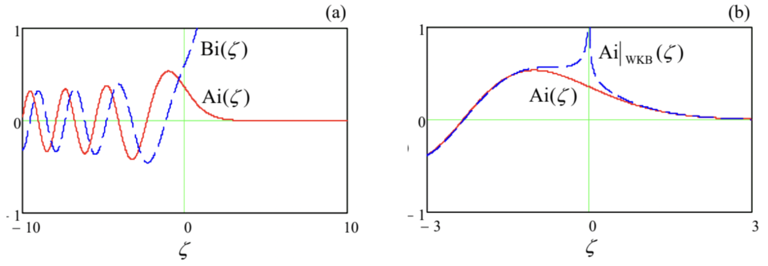
The latter function diverges at \(\zeta \rightarrow+\infty\), and thus is not suitable for our current problem (Fig. 3), while the former function has the following asymptotic behaviors at \(|\zeta|>>1\) : \[\operatorname{Ai}(\zeta) \rightarrow \frac{1}{\pi^{1 / 2}|\zeta|^{1 / 4}} \times \begin{cases}\frac{1}{2} \exp \left\{-\frac{2}{3} \zeta^{3 / 2}\right\}, & \text { for } \zeta \rightarrow+\infty \\ \sin \left\{\frac{2}{3}(-\zeta)^{3 / 2}+\frac{\pi}{4}\right\}, & \text { for } \zeta \rightarrow-\infty\end{cases}\] Now let us apply the WKB approximation to the Airy equation (101). Taking the classical turning point \((\zeta=0)\) for the lower limit, for \(\zeta>0\) we get \[\kappa^{2}(\zeta)=\zeta, \quad \kappa(\zeta)=\zeta^{1 / 2}, \quad \int_{0}^{\zeta} \kappa\left(\zeta^{\prime}\right) d \zeta^{\prime}=\frac{2}{3} \zeta^{3 / 2},\] i.e. exactly the exponent in the top line of Eq. (102). Making a similar calculation for \(\zeta<0\), with the natural assumption \(|b|=|a|\) (full reflection from the potential step), we arrive at the following result: \[\operatorname{Ai}_{\mathrm{WKB}}(\zeta)=\frac{1}{|\zeta|^{1 / 4}} \times \begin{cases}c^{\prime} \exp \left\{-\frac{2}{3} \zeta^{3 / 2}\right\}, & \text { for } \zeta>0, \\ a^{\prime} \sin \left\{\frac{2}{3}(-\zeta)^{3 / 2}+\varphi\right\}, & \text { for } \zeta<0 .\end{cases}\] This approximation differs from the exact solution at small values of \(\zeta\), i.e. close to the classical turning point \(-\) see Fig. \(9 \mathrm{~b}\). However, at \(|\zeta|>>1\), Eqs. (104) describe the Airy function exactly, provided that \[\varphi=\frac{\pi}{4}, \quad c^{\prime}=\frac{a^{\prime}}{2} .\] These connection formulas may be used to rewrite Eq. (104) as \[\mathrm{Ai}_{\mathrm{wKB}}(\zeta)=\frac{a^{\prime}}{2|\zeta|^{1 / 4}} \times\left\{\frac{\exp \left\{-\frac{2}{3} \zeta^{3 / 2}\right\},}{\frac{1}{i}\left[\exp \left\{+i \frac{2}{3} \zeta^{3 / 2}+i \frac{\pi}{4}\right\}-\exp \left\{-i \frac{2}{3} \zeta^{3 / 2}-i \frac{\pi}{4}\right\}\right],} \quad \text { for } \zeta<0,\right.\] and hence may be described by the following two simple mnemonic rules:

(i) If the classical turning point is taken for the lower limit in the WKB integrals in the classically allowed and the classically forbidden regions, then the moduli of the quasi-amplitudes of the exponents are equal.

(ii) Reflecting from a "soft" potential step, the wavefunction acquires an additional phase shift \(\Delta \varphi=\pi / 2\), if compared with its reflection from a "hard", infinitely high potential wall located at point \(x_{\mathrm{c}}\) (for which, according to Eq. (63) with \(\kappa=0\), we have \(B=-A\) ).

In order for the connection formulas (105)-(106) to be valid, deviations from the linear approximation \((99)\) of the potential profile should be relatively small within the region where the WKB approximation differs from the exact Airy function: \(|\zeta| \sim 1\), i.e. \(\left|x-x_{\mathrm{c}}\right| \sim x_{0}\). These deviations may be estimated using the next term of the Taylor expansion, dropped in Eq. (99): \(\left(d^{2} U / d^{2} x\right)\left(x-x_{\mathrm{c}}\right)^{2} / 2\). As a result, the condition of validity of the connection formulas (i.e. of the "softness" of the reflecting potential profile) may be expressed as \(\left|d^{2} U / d^{2} x\right|<<|d U / d x|\) at \(x \approx x_{\mathrm{c}}-\) meaning the \(\sim x_{0}-\) wide vicinity of the point \(x_{\mathrm{c}}\) ). With the account of Eq. (100) for \(x_{0}\), this condition becomes \[\left|\frac{d^{2} U}{d x^{2}}\right|_{x \approx x_{\mathrm{c}}}^{3}<<\frac{2 m}{\hbar^{2}}\left(\frac{d U}{d x}\right)_{x \approx x_{\mathrm{c}}}^{4}\] As an example of a very useful application of the WKB approximation, let us use the connection formulas to calculate the energy spectrum of a 1D particle in a soft 1D potential well (Fig. 10).

Fig. 2.10. The WKB treatment of an eigenstate of a particle in a soft \(1 \mathrm{D}\) potential well.

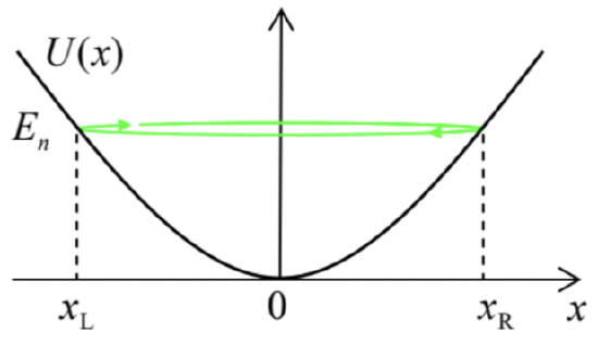
As was discussed in Sec. 1.7, we may consider the standing wave describing an eigenfunction \(\psi_{n}\) (corresponding to an eigenenergy \(E_{n}\) ) as a sum of two traveling de Broglie waves going back and forth between the walls, being sequentially reflected from each of them. Let us apply the WKB approximation to such traveling waves. First, according to Eq. (94), propagating from the left classical turning point \(x_{\mathrm{L}}\) to the right such point \(x_{R}\), it acquires the phase change \[\Delta \varphi_{\rightarrow}=\int_{x_{\mathrm{L}}}^{x_{\mathrm{R}}} k(x) d x .\] At the reflection from the soft wall at \(x_{R}\), according to the mnemonic rule (ii), the wave acquires an additional shift \(\pi / 2\). Now, traveling back from \(x_{\mathrm{R}}\) to \(x_{\mathrm{L}}\), the wave gets a shift similar to one given by Eq. (108): \(\Delta \varphi_{\leftarrow}=\Delta \varphi_{\rightarrow}\). Finally, at the reflection from \(x_{\mathrm{L}}\) it gets one more \(\pi / 2\)-shift. Summing up all these contributions at the wave’s roundtrip, we may write the self-consistency condition (that the wavefunction "catches its own tail with its teeth") in the form \[\Delta \varphi_{\text {total }} \equiv \Delta \varphi_{\rightarrow}+\frac{\pi}{2}+\Delta \varphi_{\leftarrow}+\frac{\pi}{2} \equiv 2 \int_{x_{\mathrm{L}}}^{x_{\mathrm{R}}} k(x) d x+\pi=2 \pi n, \quad \text { with } n=1,2, \ldots\] Rewriting this result in terms of the particle’s momentum \(p(x)=\hbar k(x)\), we arrive at the so-called WilsonSommerfeld (or "Bohr-Sommerfeld") quantization rule \[\oint_{C} p(x) d x=2 \pi \hbar\left(n-\frac{1}{2}\right),\] where the closed path \(C\) means the full period of classical motion. \({ }^{24}\)

Let us see what does this quantization rule give for the very important particular case of a quadratic potential profile of a harmonic oscillator of frequency \(\omega_{0}\). In this case, \[U(x)=\frac{m}{2} \omega_{0}^{2} x^{2},\] and the classical turning points (where \(U(x)=E\) ) are the roots of a simple equation \[\frac{m}{2} \omega_{0}^{2} x_{\mathrm{c}}^{2}=E_{n}, \quad \text { so that } x_{\mathrm{R}}=\frac{1}{\omega_{0}}\left(\frac{2 E_{n}}{m}\right)^{1 / 2}>0, \quad x_{\mathrm{L}}=-x_{\mathrm{R}}<0 .\] Due to the potential’s symmetry, the integration required by Eq. (110) is also simple: \[\begin{aligned} \int_{x_{\mathrm{L}}}^{x_{\mathrm{R}}} p(x) d x &=\int_{x_{\mathrm{L}}}^{x_{\mathrm{R}}}\left\{2 m\left[E_{n}-U(x)\right]\right\}^{1 / 2} d x \equiv\left(2 m E_{n}\right)^{1 / 2} 2 \int_{0}^{x_{\mathrm{R}}}\left(1-\frac{x^{2}}{x_{\mathrm{R}}^{2}}\right)^{1 / 2} d x \\ & \equiv\left(2 m E_{n}\right)^{1 / 2} 2 x_{\mathrm{R}} \int_{0}^{1}\left(1-\xi^{2}\right)^{1 / 2} d \xi=\left(2 m E_{n}\right)^{1 / 2} 2 x_{\mathrm{R}} \frac{\pi}{4} \equiv \frac{\pi E_{n}}{\omega_{0}} \end{aligned}\] so that Eq. (110) yields \[E_{n}=\hbar \omega_{0}\left(n^{\prime}+\frac{1}{2}\right), \quad \text { with } n^{\prime} \equiv n-1=0,1,2, \ldots .\] To estimate the validity of this result, we have to check the condition (96) at all points of the classically allowed region, and Eq. (107) at the turning points. The checkup shows that both conditions are valid only for \(n \gg>1\). However, we will see in Sec. 9 below that Eq. (114) is actually exactly correct for all energy levels - thanks to special properties of the potential profile (111).

Now let us use the mnemonic rule (i) to examine particle’s penetration into the classically forbidden region of an abrupt potential step of a height \(U_{0}>E\). For this case, the rule, i.e. the second of Eqs. (105), yields the following relation of the quasi-amplitudes in Eqs. (94) and (98): \(|c|=|a| / 2\). If we now naively applied this relation to the sharp step sketched in Fig. 4, forgetting that it does not satisfy Eq. (107), we would get the following relation of the full amplitudes, defined by Eqs. (55) and (58): \[\left|\frac{C}{\kappa}\right|=\frac{1}{2}\left|\frac{A}{k}\right| . \quad \text { (WRONG!) }\] This result differs from the correct Eq. (63), and hence we may expect that the WKB approximation’s prediction for more complex potentials, most importantly for tunneling through a soft potential barrier (Fig. 11) should be also different from the exact result (71) for the rectangular barrier shown in Fig. 6 .

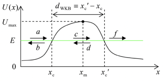Fig. 2.11. Tunneling through a soft 1D potential barrier.

In order to analyze tunneling through such a soft barrier, we need (just as in the case of a rectangular barrier) to take unto consideration five partial waves, but now they should be taken in the WKB form: \[\psi_{\mathrm{WKB}}= \begin{cases}\frac{a}{k^{1 / 2}(x)} \exp \left\{\frac{c}{\kappa^{1 / 2}(x)} \exp \left\{-\int^{x} k\left(x^{\prime}\right) d x^{\prime}\right\}+\frac{b}{k^{1 / 2}(x)} \exp \left\{-i \int^{x} k\left(x^{\prime}\right) d x^{\prime}\right\},\right. & \text { for } x<x_{\mathrm{c}}, \\ \frac{f}{k^{1 / 2}(x)} \exp \left\{\frac{d}{i \int k\left(x^{\prime}\right) d x^{\prime}}\right\}, & \text { for } x_{\mathrm{c}}<x<x_{\mathrm{c}}^{\prime}, \\ & \text { for } x_{\mathrm{c}}^{\prime}<x,\end{cases}\] where the lower limits of integrals are arbitrary (each within the corresponding range of \(x\) ). Since on the right of the left classical point, we have two exponents rather than one, and on the right of the second point, one traveling waves rather than two, the connection formulas (105) have to be generalized, using asymptotic formulas not only for \(\operatorname{Ai}(\zeta)\), but also for the second \(\operatorname{Airy}\) function, \(\operatorname{Bi}(\zeta)\). The analysis, absolutely similar to that carried out above (though naturally a bit bulkier), \({ }^{25}\) gives a remarkably simple result: \[\mathscr{T}_{\mathrm{WKB}} \equiv\left|\frac{f}{a}\right|^{2}=\exp \left\{-2 \int_{x_{\mathrm{c}}}^{x_{\mathrm{c}}^{\prime}} \kappa(x) d x\right\} \equiv \exp \left\{-\frac{2}{\hbar} \int_{x_{\mathrm{c}}}^{x_{\mathrm{c}}^{\prime}}(2 m[U(x)-E])^{1 / 2} d x\right\}\] with the pre-exponential factor equal to 1 - the fact which might be readily expected from the mnemonic rule (i) of the connection formulas.

This formula is broadly used in applied quantum mechanics, despite the approximate character of its pre-exponential coefficient for insufficiently soft barriers that do not satisfy Eq. (107). For example, Eq. (80) shows that for a rectangular barrier with thickness \(d \gg>\delta\), the WKB approximation (117) with \(d_{\mathrm{WKB}}=d\) underestimates \(\mathscr{T}\) by a factor of \(\left[4 k \kappa /\left(k^{2}+\kappa^{2}\right)\right]^{2}-\) equal, for example, 4 , if \(k=\kappa\), i.e. if \(U_{0}=2 E\). However, on the appropriate logarithmic scale (see Fig. 7b), such a factor, smaller than an order of magnitude, is just a small correction.

Note also that when \(E\) approaches the barrier’s top \(U_{\max }\) (Fig. 11), the points \(x_{\mathrm{c}}\) and \(x_{\mathrm{c}}\) ’ merge, so that according to Eq. (117), \(\mathscr{T}_{\text {WKB }} \rightarrow 1\), i.e. the particle reflection vanishes at \(E=U_{\text {max }}\). So, the WKB approximation does not describe the effect of the over-barrier reflection at \(E>U_{\max }\). (This fact could be noticed already from Eq. (95): in the absence of the classical turning points, the WKB probability current is constant for any barrier profile.) This conclusion is incorrect even for apparently smooth barriers where one could naively expect the WKB approximation to work perfectly. Indeed, near the point \(x=x_{\mathrm{m}}\) where the potential reaches maximum (i.e. \(U\left(x_{\mathrm{m}}\right)=U_{\max }\) ), we may always approximate any smooth function \(U(x)\) with the quadratic term of the Taylor expansion, i.e. with an inverted parabola: \[U(x) \approx U_{\max }-\frac{m \omega_{0}^{2}\left(x-x_{\mathrm{m}}\right)^{2}}{2} .\] Calculating derivatives \(d U / d x\) and \(d^{2} U / d x^{2}\) of this function and plugging them into the condition \((107)\), we may see that the WKB approximation is only valid if \(\left|U_{\max }-E\right| \gg>\hbar \omega_{0}\). Just for the reader’s reference, an exact analysis of tunneling through the barrier (118) gives the following Kemble formula: 26 \[\mathscr{T}=\frac{1}{1+\exp \left\{-2 \pi\left(E-U_{\max }\right) / \hbar \omega_{0}\right\}},\] valid for any sign of the difference \(\left(E-U_{\max }\right) .\) This formula describes a gradual approach of \(\mathscr{T}\) to 1 , i.e. a gradual reduction of reflection, at the particle energy’s increase, with \(\mathscr{T}=1 / 2\) at \(E=U_{\max }\).

The last remark of this section: the WKB approximation opens a straight way toward an alternative formulation of quantum mechanics, based on the Feynman path integral. However, I will postpone its discussion until a more compact notation has been introduced in Chapter \(4 .\)

---

\({ }^{19}\) Quantitative conditions of the "softness" will be formulated later in this section.

\({ }^{20}\) Philosophically, this space-domain method is very close to the time-domain van der Pol method in classical mechanics, and the very similar rotating wave approximation (RWA) in quantum mechanics - see, e.g., CM Secs. \(5.2-5.5\), and also Secs. \(6.5,7.6,9.2\), and \(9.4\) of this course.

\({ }^{21}\) For certainty, I will use the discretion given by Eq. (82) to define \(k(x)\) as the positive root of its right-hand side.

\({ }^{22}\) An alternative way to solve the connection problem, without involving the Airy functions but using an analytical extension of WKB formulas to the complex-argument plane, may be found, e.g., in Sec. 47 of the textbook by L. Landau and E. Lifshitz, Quantum Mechanics, Non-Relativistic Theory, 3rd ed. Pergamon, \(1977 .\)

\({ }^{23}\) Note the following (exact) integral formulas,

\(\operatorname{Ai}(\zeta)=\frac{1}{\pi} \int_{0}^{\infty} \cos \left(\frac{\xi^{3}}{3}+\zeta \xi\right) d \xi, \quad \operatorname{Bi}(\zeta)=\frac{1}{\pi} \int_{0}^{\infty}\left[\exp \left\{-\frac{\xi^{3}}{3}+\zeta \xi\right\}+\sin \left(\frac{\xi^{3}}{3}+\zeta \xi\right)\right] d \xi,\)

frequently more convenient for practical calculations of the Airy functions than the differential equation (101).

\({ }^{24}\) Note that at the motion in more than one dimension, a closed classical trajectory may have no classical turning points. In this case, the constant \(1 / 2\), arising from the turns, should be dropped from Eqs. (110) written for the scalar product \(\mathbf{p}(\mathbf{r}) \cdot d \mathbf{r}\) - the so-called Bohr quantization rule. It was suggested by N. Bohr as early as 1913 as an interpretation of Eq. (1.8) for the circular motion of the electron around the proton, while its 1D modification (110) is due to W. Wilson (1915) and A. Sommerfeld (1916).

\({ }^{25}\) For the most important case \(\mathcal{T}_{\text {WKB }}<<1\), Eq. (117) may be simply derived from Eqs. (105)-(106) - the exercise left for the reader.

\({ }^{26}\) This formula was derived (in a more general form, valid for an arbitrary soft potential barrier) by E. Kemble in 1935. In some communities, it is known as the "Hill-Wheeler formula", after D. Hill and J. Wheeler’s 1953 paper in that the Kemble formula was spelled out for the quadratic profile (118). Note that mathematically Eq. (119) is similar to the Fermi distribution in statistical physics, with an effective temperature \(T_{\text {ef }}=\hbar \omega_{0} / 2 \pi k_{\text {B }}\). This coincidence has some curious implications for the Fermi particle tunneling statistics.