2.4: Exercise Problems

2.1. The initial wave packet of a free 1D particle is described by Eq. (20):

$$\Psi(x, 0)=\int a_{k} e^{i k x} d k .$$ (i) Obtain a compact expression for the expectation value $\langle p\rangle$ of the particle’s momentum at an arbitrary moment $t>0$.

(ii) Calculate $\langle p\rangle$ for the case when the function $\left|a_{k}\right|^{2}$ is symmetric with respect to some value $k_{0}$.

2.2. Calculate the function $a_{k}$ defined by Eq. (20), for the wave packet with a rectangular spatial envelope:

$$\Psi(x, 0)= \begin{cases}C \exp \left\{i k_{0} x\right\}, & \text { for }-a / 2 \leq x \leq+a / 2, \\ 0, & \text { otherwise } .\end{cases}$$ Analyze the result in the limit $k_{0} a \rightarrow \infty$.

2.3. Prove Eq. (49) for the 1D propagator of a free quantum particle, starting from Eq. (48).

2.4. Express the $1 \mathrm{D}$ propagator defined by Eq. (44), via the eigenfunctions and eigenenergies of a particle moving in an arbitrary stationary potential $U(x)$.

2.5. Calculate the change of the wavefunction of a $1 \mathrm{D}$ particle, resulting from a short pulse of an external classical force that may be approximated by the delta function: ${ }^{97}$

$$F(t)=P \delta(t) \text {. }$$ 2.6. Calculate the transparency $\mathscr{T}$ of the rectangular potential barrier (68), $$U(x)= \begin{cases}0, & \text { for } x<-d / 2 \\ U_{0}, & \text { for }-d / 2<x<+d / 2 \\ 0, & \text { for } d / 2<x,\end{cases}$$ for a particle of energy $E>U_{0}$. Analyze and interpret the result, taking into account that $U_{0}$ may be either positive or negative. (In the latter case, we are speaking about the particle’s passage over a rectangular potential well of a finite depth $\left|U_{0}\right|$.)

2.7. Prove Eq. (117) for the case $\mathcal{T}_{\mathrm{WKB}}<<1$, using the connection formulas (105).

2.8. Spell out the stationary wavefunctions of a harmonic oscillator in the WKB approximation, and use them to calculate the expectation values $\left\langle x^{2}\right\rangle$ and $\left\langle x^{4}\right\rangle$ for the eigenstate number $\left.n\right\rangle>1 .$

2.9. Use the WKB approximation to express the expectation value of the kinetic energy of a 1D particle confined in a soft potential well, in its $n^{\text {th }}$ stationary state, via the derivative $d E_{n} / d n$, for $n>>1$.

2.10. Use the WKB approximation to calculate the transparency $\mathscr{T}$ of the following triangular potential barrier:

$$U(x)=\left\{\begin{array}{cc} 0, & \text { for } x<0 \\ U_{0}-F x, & \text { for } x>0 \end{array}\right.$$ with $F, U_{0}>0$, as a function of the incident particle’s energy $E$.

Hint: Be careful with the sharp potential step at $x=0$.

2.11. Prove that the symmetry of the 1D scattering matrix S describing an arbitrary timeindependent scatterer, allows its representation in the form (127).

2.12. Prove the universal relations between elements of the 1D transfer matrix $\mathrm{T}$ of a stationary (but otherwise arbitrary) scatterer, mentioned in Sec. $5 .$

2.13. A 1D particle had been localized in a very narrow and deep potential well, with the "energy area" $\int \overline{U(x)} d x$ equal to $-w$, where $w>0$. Then (say, at $t=0$ ) the well’s bottom is suddenly lifted up, so that the particle becomes completely free. Calculate the probability density, $w(k)$, to find the particle in a state with a certain wave number $k$ at $t>0$, and the total final energy of the system.

2.14. Calculate the lifetime of the metastable localized state of a $1 \mathrm{D}$ particle in the potential

$$U(x)=-w \delta(x)-F x, \quad \text { with } w>0,$$ using the WKB approximation. Formulate the condition of validity of the result.

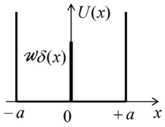
2.15. Calculate the energy levels and the corresponding eigenfunctions of a 1D particle placed into a flat-bottom potential well of width $2 a$, with infinitely-high hard walls, and a transparent, short potential barrier in the middle - see the figure on the right. Discuss particle dynamics in the limit when $w$ is very large but still finite.

2.16. ${ }^{*}$ Consider a symmetric system of two potential wells of the type shown in Fig. 21, but with $U(0)=U(\pm \infty)=0-$ see the figure on the right. What is the sign of the well interaction force due to their sharing a quantum particle of mass $m$, for the cases when the particle is in:

(i) a symmetric localized eigenstate: $\psi_{\mathrm{S}}(-x)=\psi_{\mathrm{s}}(x)$ ?

(ii) an antisymmetric localized eigenstate: $\psi_{\mathrm{A}}(-x)=-\psi_{\mathrm{A}}(x)$ ?

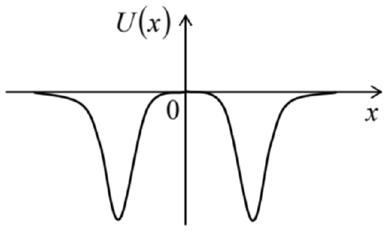
Use an alternative approach to verify your result for the particular case of delta-functional wells.

2.17. Derive and analyze the characteristic equation for localized eigenstates of a 1D particle in a rectangular potential well of a finite depth (see the figure on the right):

$$U(x)=\left\{\begin{aligned} -U_{0}, & \text { for }|x| \leq a / 2, \\ 0, & \text { otherwise } \end{aligned}\right.$$

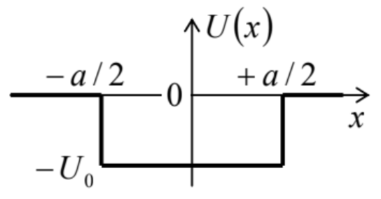
In particular, calculate the number of localized states as a function of well’s width $a$, and explore the limit $U_{0}<<\hbar^{2} / 2 m a^{2}$. 2.18. Calculate the energy of a $1 \mathrm{D}$ particle localized in a potential well of an arbitrary shape $U(x)$, provided that its width $a$ is finite, and the average depth is very small:

$$|\bar{U}|<<\frac{\hbar^{2}}{2 m a^{2}}, \quad \text { where } \bar{U} \equiv \frac{1}{a} \int_{\text {well }} U(x) d x$$ 2.19. A particle of mass $m$ is moving in a field with the following potential: $$U(x)=U_{0}(x)+w \delta(x) \text {, }$$ where $U_{0}(x)$ is a smooth, symmetric function with $U_{0}(0)=0$, growing monotonically at $x \rightarrow \pm \infty$.

(i) Use the WKB approximation to derive the characteristic equation for the particle’s energy spectrum, and

(ii) semi-quantitatively describe the spectrum’s evolution at the increase of $|W|$, for both signs of this parameter.

Make both results more specific for the quadratic-parabolic potential (111): $U_{0}(x)=m \omega_{0}^{2} x^{2} / 2$.

$\underline{2.20}$. Prove Eq. (189), starting from Eq. (188).

2.21. For the problem discussed at the beginning of Sec. 7, i.e. the 1D particle’s motion in an infinite Dirac comb potential shown in Fig. 24 ,

$$U(x)=w \sum_{j=-\infty}^{+\infty} \delta(x-j a), \quad \text { with } w>0,$$ (where $j$ takes integer values), write explicit expressions for the eigenfunctions at the very bottom and at the very top of the lowest energy band. Sketch both functions.

2.22. A 1D particle of mass $m$ moves in an infinite periodic system of very narrow and deep potential wells that may be described by delta functions:

$$U(x)=w \sum_{j=-\infty}^{+\infty} \delta(x-j a), \quad \text { with } w<0 .$$ (i) Sketch the energy band structure of the system for very small and very large values of the potential well’s "weight" $|w|$, and

(ii) calculate explicitly the ground state energy of the system in these two limits.

2.23. For the system discussed in the previous problem, write explicit expressions for the eigenfunctions of the system, corresponding to:

(i) the bottom of the lowest energy band,

(ii) the top of that band, and

(iii) the bottom of each higher energy band.

Sketch these functions.

$\underline{2.24}$. The $1 \mathrm{D}$ "crystal" analyzed in the last two problems, now extends only to $x>0$, with a sharp step to a flat potential plateau at $x<0$ :

$$U(x)= \begin{cases}w \sum_{j=1}^{+\infty} \delta(x-j a), & \text { with } w<0, \\ U_{0}>0, & \text { for } x>0,\end{cases}$$ Prove that the system can have a set of the so-called Tamm states, localized near the "surface" $x=0$, and calculate their energies in the limit when $U_{0}$ is very large but finite. (Quantify this condition.) ${ }^{98}$

2.25. Calculate the whole transfer matrix of the rectangular potential barrier, specified by Eq. (68), for particle energies both below and above $U_{0}$.

2.26. Use the results of the previous problem to calculate the transfer matrix of one period of the periodic Kronig-Penney potential shown in Fig. 31b.

2.27. Using the results of the previous problem, derive the characteristic equations for particle’s motion in the periodic Kronig-Penney potential, for both $E<U_{0}$ and $E>U_{0}$. Try to bring the equations to a form similar to that obtained in Sec. 7 for the delta-functional barriers - see Eq. (198). Use the equations to formulate the conditions of applicability of the tight-binding and weak-potential approximations, in terms of the system’s parameters, and the particle’s energy $E$.

2.28. For the Kronig-Penney potential, use the tight-binding approximation to calculate the widths of the allowed energy bands. Compare the results with those of the previous problem (in the corresponding limit).

2.29. For the same Kronig-Penney potential, use the weak-potential limit formulas to calculate the energy gap widths. Again, compare the results with those of Problem 27 , in the corresponding limit.

2.30. 1D periodic chains of atoms may exhibit what is called the Peierls instability, leading to the Peierls transition to a phase in which atoms are slightly displaced, from the exact periodicity, by alternating displacements $\Delta x_{j}=(-1)^{j} \Delta x$, with $\Delta x<<a$, where $j$ is the atom’s number in the chain, and $a$ is its initial period. These displacements lead to the alternation of the coupling amplitudes $\delta_{n}$ (see Eq. (204)) between close values $\delta_{n}^{+}$and $\delta_{n}^{-}$. Use the tight-binding approximation to calculate the resulting change of the $n^{\text {th }}$ energy band, and discuss the result.

2.31. " Use Eqs. (1.73)-(1.74) of the lecture notes to derive Eq. (252), and discuss the relation between these Bloch oscillations and the Josephson oscillations of frequency (1.75).

2.32. A 1D particle of mass $m$ is placed to the following triangular potential well:

$$U(x)=\left\{\begin{array}{ll} +\infty, & \text { for } x<0, \\ F x, & \text { for } x>0, \end{array} \text { with } F>0\right. \text {. }$$ (i) Calculate its energy spectrum using the WKB approximation.

(ii) Estimate the ground state energy using the variational method, with two different trial functions.

(iii) Calculate the three lowest energy levels, and also the $10^{\text {th }}$ level, with an accuracy better than $0.1 \%$, from the exact solution of the problem.

(iv) Compare and discuss the results.

Hint: The values of the first zeros of the Airy function, necessary for Task (iii), may be found in many math handbooks, for example, in Table $9.9 .1$ of the online version of the collection edited by Abramowitz and Stegun - see MA Sec. 16(i).

$\underline{2.33}$. Use the variational method to estimate the ground state energy $E_{\mathrm{g}}$ of a particle in the following potential well:

$$U(x)=-U_{0} \exp \left\{-\alpha x^{2}\right\}, \quad \text { with } \alpha>0, \text { and } U_{0}>0 .$$ Spell out the results in the limits of small and large $U_{0}$, and give their interpretation.

2.34. For a 1D particle of mass $m$, placed to a potential well with the following profile,

$$U(x)=a x^{2 s} \text {, with } a>0 \text {, and } s>0 \text {, }$$ (i) calculate its energy spectrum using the WKB approximation, and

(ii) estimate the ground state energy using the variational method.

Compare the ground-state energy results for the parameter $s$ equal to $1,2,3$, and 100 .

2.35. Use the variational method to estimate the $1^{\text {st }}$ excited state of the $1 \mathrm{D}$ harmonic oscillator.

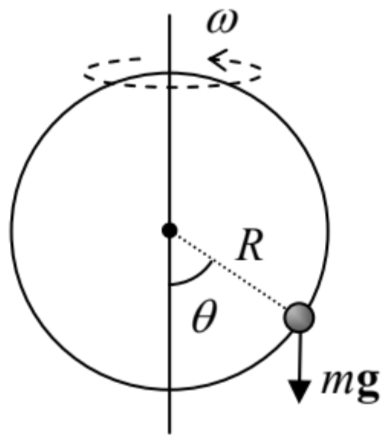
2.36. Assuming the quantum effects to be small, calculate the lower part of the energy spectrum of the following system: a small bead of mass $m$, free to move without friction along a ring of radius $R$, which is rotated about its vertical diameter with a constant angular velocity $\omega-$ see the figure on the right. Formulate a quantitative condition of validity of your results.

Hint: This system was used as the analytical mechanics’ "testbed problem" in the CM part of this series, and the reader is welcome to use any relations derived there.

2.37. A 1D harmonic oscillator, with mass $m$ and frequency $\omega_{0}$, had been in its ; then an additional force $F$ was suddenly applied, and after that kept constant. Calculate the probability of the oscillator staying in its ground state.

2.38. A 1D particle of mass $m$ has been placed to a quadratic potential well (111),

$$U(x)=\frac{m \omega_{0}^{2} x^{2}}{2},$$ and allowed to relax into the ground state. At $t=0$, the well was fast accelerated to move with velocity $v$, without changing its profile, so that at $t \geq 0$ the above formula for $U$ is valid with the replacement $x \rightarrow$ $x^{\prime} \equiv x-v t$. Calculate the probability for the system to still be in the ground state at $t>0$. 2.39. Initially, a 1D harmonic oscillator was in its ground state. At a certain moment of time, its spring constant $\kappa$ is abruptly increased so that its frequency $\omega_{0}=(\kappa / m)^{1 / 2}$ is increased by a factor of $\alpha$, and then is kept constant at the new value. Calculate the probability that after the change, the oscillator is still in its ground state.

2.40. A 1D particle is placed into the following potential well:

$$U(x)= \begin{cases}+\infty, & \text { for } x<0, \\ m \omega_{0}^{2} x^{2} / 2, & \text { for } x \geq 0 .\end{cases}$$ (i) Find its eigenfunctions and eigenenergies.

(ii) This system had been let to relax into its ground state, and then the potential wall at $x<0$ was rapidly removed so that the system was instantly turned into the usual harmonic oscillator (with the same $m$ and $\omega_{0}$ ). Find the probability for the oscillator to remain in its ground state.

2.41. Prove the following formula for the propagator of the 1D harmonic oscillator:

$$G\left(x, t ; x_{0}, t_{0}\right)=\left(\frac{m \omega_{0}}{2 \pi i \hbar \sin \left[\omega_{0}\left(t-t_{0}\right)\right]}\right)^{1 / 2} \exp \left\{\frac{i m \omega_{0}}{2 \hbar \sin \left[\omega_{0}\left(t-t_{0}\right)\right]}\left[\left(x^{2}+x_{0}^{2}\right) \cos \left[\omega_{0}\left(t-t_{0}\right)\right]-2 x x_{0}\right]\right\} .$$ Discuss the relation between this formula and the propagator of a free 1D particle.

2.42. In the context of the Sturm oscillation theorem mentioned in Sec. 9, prove that the number of eigenfunction’s zeros of a particle confined in an arbitrary but finite potential well always increases with the corresponding eigenenergy.

Hint: You may like to use the suitably modified Eq. (186).

2.43. ${ }^{*}$ Use the WKB approximation to calculate the lifetime of the metastable ground state of a 1D particle of mass $m$ in the "pocket" of the potential profile

$$U(x)=\frac{m \omega_{0}^{2}}{2} x^{2}-\alpha x^{3} .$$ Contemplate the significance of this problem.

---

${ }_{97}$ The constant $P$ is called the force’s impulse. (In higher dimensionalities, it is a vector - just as the force is.)

${ }_{98}$ In applications to electrons in solid-state crystals, the delta-functional potential wells model the attractive potentials of atomic nuclei, while $U_{0}$ represents the workfunction, i.e. the energy necessary for the extraction of an electron from the crystal to the free space - see, e.g., Sec. 1.1(ii), and also EM Sec. $2.6$ and SM Sec. 6.3.