7.1: Open Systems, and the Density Matrix

All the way until the last part of the previous chapter, we have discussed quantum systems isolated from their environment. Indeed, from the very beginning, we have assumed that we are dealing with the statistical ensembles of systems as similar to each other as only allowed by the laws of quantum mechanics. Each member of such an ensemble, called pure or coherent, may be described by the same state vector \(|\alpha\rangle\) - in the wave mechanics case, by the same wavefunction \(\Psi_{\alpha}\). Even the discussion at the end of the last chapter, in which one component system (in Fig. 6.13, system \(b\) ) may be used as a model of the environment of its counterpart (system \(a\) ), was still based on the assumption of a pure initial state (6.143) of the composite system. If the interaction of the two components of such a system is described by a certain Hamiltonian (the one given by Eq. (6.145) for example), and the energy spectrum of each component system is discrete, for state \(\alpha\) of the composite system at an arbitrary instant we may write \[|\alpha\rangle=\sum_{n} \alpha_{n}|n\rangle=\sum_{n} \alpha_{n}\left|n_{a}\right\rangle \otimes\left|n_{b}\right\rangle,\] with a unique correspondence between the eigenstates \(n_{a}\) and \(n_{b}\).

However, in many important cases, our knowledge of a quantum system’s state is even less complete. \(^{2}\) These cases fall into two categories. The first case is when a relatively simple quantum system \(s\) of our interest (say, an electron or an atom) is in a weak \(^{3}\) but substantial contact with its environment \(e\) - here understood in the most general sense, say, as all the whole Universe less system \(s\) - see Fig. 1. Then there is virtually no chance of making two or more experiments with exactly the same composite system because that would imply a repeated preparation of the whole environment (including the experimenter :-) in a certain quantum state - a rather challenging task, to put it mildly. Then it makes much more sense to consider a statistical ensemble of another kind - a mixed ensemble, with random states of the environment, though possibly with its macroscopic parameters (e.g., temperature, pressure, etc.) known with high precision. Such ensembles will be the focus of the analysis in this chapter

Much of this analysis will pertain also to another category of cases - when the system of our interest is isolated from its environment, at present, with acceptable precision, but our knowledge of its state is still incomplete for some other reason. Most typically, the system could be in contact with its environment at earlier times, and its reduction to a pure state is impracticable. So, this second category of cases may be considered as a particular case of the first one, and may be described by the results of its analysis, with certain simplifications - which will be spelled out in appropriate places of my narrative.

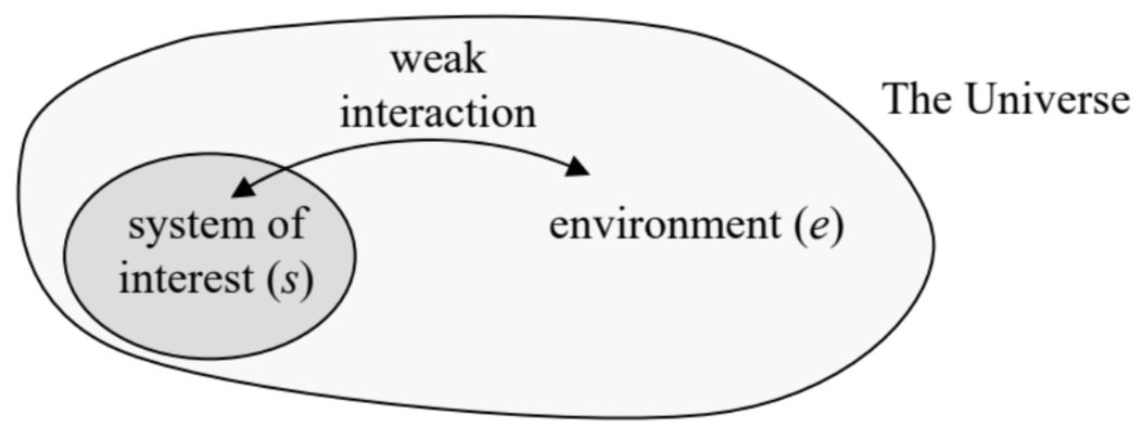Fig. 7.1. A quantum system and its environment (VERY schematically :-).

In classical physics, the analysis of mixed statistical ensembles is based on the notion of the probability \(W\) (or the probability density \(w\) ) of each detailed ("microscopic") state of the system of interest. \({ }^{4}\) Let us see how such an ensemble may be described in quantum mechanics. In the case when the coupling between the system of our interest and its environment is so weak that they may be clearly separated, we can still use state vectors of their states, defined in completely different Hilbert spaces. Then the most general quantum state of the whole Universe, still assumed to be pure, \({ }^{5}\) may be described as the following linear superposition: \[|\alpha\rangle=\sum_{j, k} \alpha_{j k}\left|s_{j}\right\rangle \otimes\left|e_{k}\right\rangle .\] The "only" difference of such a state from the superposition described by Eq. (1), is that there is no one-to-one correspondence between the states of our system and its environment. In other words, a certain quantum state \(s_{j}\) of the system of interest may coexist with different states \(e_{k}\) of its environment. This is exactly the quantum-mechanical description of a mixed state of the system \(s\).

Of course, the huge size of the Hilbert space of the environment, i.e. of the number of the \(\left|e_{k}\right\rangle\) factors in the superposition (2), strips us of any practical opportunity to make direct calculations using that sum. For example, according to the basic Eq. (4.125), to find the expectation value of an arbitrary observable \(A\) in the state (2), we would need to calculate the long bracket \[\langle A\rangle=\langle\alpha|\hat{A}| \alpha\rangle \equiv \sum_{j, j^{\prime} ; k, k^{\prime}} \alpha^{*} \alpha_{j k^{\prime}}\left\langle e_{k}\left|\otimes\left\langle s_{j}|\hat{A}| s_{j^{\prime}}\right\rangle \otimes\right| e_{k^{\prime}}\right\rangle .\] Even if we assume that each of the sets \(\{s\}\) and \(\{e\}\) is full and orthonormal, Eq. (3) still includes a double sum over the enormous basis state set of the environment!

However, let us consider a limited, but the most important subset of operators - those of intrinsic observables, which depend only on the degrees of freedom of the system of our interest \((s)\). These operators do not act upon the environment’s degrees of freedom, and hence in Eq. (3), we may move the environment’s bra-vectors \(\left\langle e_{k}\right|\) over all the way to the ket-vectors \(\left|e_{k^{\prime}}\right\rangle\). Assuming, again, that the set of environmental eigenstates is full and orthonormal, Eq. (3) is now reduced to

\[\langle A\rangle=\sum_{j, j^{\prime} ; k, k^{\prime}} \alpha_{j k}^{*} \alpha_{j^{\prime} k^{\prime}}\left\langle s_{j}|\hat{A}| s_{j^{\prime}}\right\rangle\left\langle e_{k} \mid e_{k^{\prime}}\right\rangle=\sum_{i j^{\prime}} A_{i j^{\prime}} \sum_{k} \alpha_{j k}^{*} \alpha_{j^{\prime} k} .\] This is already a big relief because we have "only" a single sum over \(k\), but the main trick is still ahead. After the summation over \(k\), the second sum in the last form of Eq. (4) is some function \(w\) of the indices \(j\) and \(j\) ’, so that, according to Eq. (4.96), this relation may be represented as \[\langle A\rangle=\sum_{i j^{\prime}} A_{j j^{\prime}} w_{j^{\prime} j} \equiv \operatorname{Tr}(\mathrm{Aw}),\] where the matrix w, with the elements \[w_{j j} \equiv \sum_{k} \alpha_{j k}^{*} \alpha_{j^{\prime} k}, \quad \text { i.e. } w_{j j^{\prime}} \equiv \sum_{k} \alpha_{j k} \alpha_{j^{\prime} k}^{*},\] is called the density matrix of the system. \({ }^{6}\) Most importantly, Eq. (5) shows that the knowledge of this matrix allows the calculation of the expectation value of any intrinsic observable \(A\) (and, according to the general Eqs. (1.33)-(1.34), its r.m.s. fluctuation as well, if needed), even for the very general state (2). This is why let us have a good look at the density matrix.

First of all, we know from the general discussion in Chapter 4, fully applicable to the pure state (2), the expansion coefficients in superpositions of this type may be always expressed as short brackets of the type (4.40); in our current case, we may write \[\alpha_{j k}=\left(\left\langle e_{k}\left|\otimes\left\langle s_{j}\right|\right) \mid \alpha\right\rangle .\right.\] Plugging this expression into Eq. (6), we get \[w_{i j^{\prime}} \equiv \sum_{k} \alpha_{j k} \alpha_{j^{\prime} k}^{*}=\left\langle s_{j}\left|\otimes\left(\sum_{k}\left\langle e_{k} \mid \alpha\right\rangle\left\langle\alpha \mid e_{k}\right\rangle\right) \otimes\right| s_{j^{\prime}}\right\rangle=\left\langle s_{j}|\hat{w}| s_{j^{\prime}}\right\rangle .\] We see that from the point of our system (i.e. in its Hilbert space whose basis states may be numbered by the index \(j\) only), the density matrix is indeed just the matrix of some construct, \({ }^{7}\) \[\hat{w} \equiv \sum_{k}\left\langle e_{k} \mid \alpha\right\rangle\left\langle\alpha \mid e_{k}\right\rangle,\] which is called the density (or "statistical") operator. As it follows from the definition (9), in contrast to the density matrix this operator does not depend on the choice of a particular basis \(s_{j}\) - just as all linear operators considered earlier in this course. However, in contrast to them, the density operator does depend on the composite system’s state \(\alpha\), including the state of the system \(s\) as well. Still, in the \(j\)-space it is mathematically just an operator whose matrix elements obey all relations of the bra-ket formalism.In particular, due to its definition (6), the density operator is Hermitian: \[w_{i j^{\prime}}^{*}=\sum_{k} \alpha_{j k}^{*} \alpha_{j k}=\sum_{k} \alpha_{j k} \alpha_{j k}^{*}=w_{j j}\] so that according to the general analysis of Sec. 4.3, in the Hilbert space of the system \(s\), there should be a certain basis \(\{w\}\) in that the matrix of this operator is diagonal: \[w_{i j^{\prime}} \text { in } w=w_{j} \delta_{j j^{\prime}} \text {. }\] Since any operator, in any basis, may be represented in the form (4.59), in the basis \(\{w\}\) we may write \[\hat{w}=\sum_{j}\left|w_{j}\right\rangle w_{j}\left\langle w_{j}\right|\] This expression reminds, but is not equivalent to Eq. (4.44) for the identity operator, that has been used so many times in this course, and in the basis \(w_{j}\) has the form \[\hat{I}=\sum_{j}\left|w_{j}\right\rangle\left\langle w_{j}\right| \text {. }\] In order to comprehend the meaning of the coefficients \(w_{j}\) participating in Eq. (12), let us use Eq. (5) to calculate the expectation value of any observable \(A\) whose eigenstates coincide with those of the special basis \(\{w\}\), and whose matrix is, therefore, diagonal in this basis: \[\langle A\rangle=\operatorname{Tr}(\mathrm{Aw})=\sum_{i j^{\prime}} A_{j j^{\prime}} w_{j} \delta_{j j^{\prime}}=\sum_{j} A_{j} w_{j},\] where \(A_{j}\) is just the expectation value of the observable \(A\) in the state \(w_{j}\). Hence, to comply with the general Eq. (1.37), the real \(c\)-number \(w_{j}\) must have the physical sense of the probability \(W_{j}\) of finding the system in the state \(j\). As the result, we may rewrite Eq. (12) in the form \[\hat{w}=\sum_{j}\left|w_{j}\right\rangle W_{j}\left\langle w_{j}\right| \text {. }\] In the ultimate case when only one of the probabilities (say, \(W_{j^{\prime \prime}}\) ) is different from zero, \[W_{j}=\delta_{j j^{\prime \prime}},\] the system is in a coherent (pure) state \(w_{j} "\). Indeed, it is fully described by one ket-vector \(\left|w_{j} "\right\rangle\), and we can use the general rule (4.86) to represent it in another (arbitrary) basis \(\{s\}\) as a coherent superposition

\[\ \left|w_{j^{\prime \prime}}\right\rangle=\sum_{j^{\prime}} U_{j^{\prime \prime} i^\prime}^{\dagger}\left|s_{j^{\prime}}\right\rangle=\sum_{j^{\prime}} U_{j^{\prime} j^{\prime \prime}}^{*}\left|s_{j^{\prime}}\right\rangle,\]

where \(\mathrm{U}\) is the unitary matrix of transform from the basis \(\{w\}\) to the basis \(\{s\}\). According to Eqs. (11) and (16), in such a pure state the density matrix is diagonal in the \(\{w\}\) basis, \[w_{i j^{\prime}} \mid \text { in } w=\delta_{j, j^{\prime \prime}} \delta_{j^{\prime}, j^{\prime \prime}},\] but not in an arbitrary basis. Indeed, using the general rule (4.92), we get \[w_{i j^{\prime} \mid \text { ins }}=\sum_{l, l^{\prime}} U_{j l^{\prime}}^{\dagger} w_{l l^{\prime}} \text { in } w_{l j^{\prime}}=U_{i j^{\prime \prime}}^{\dagger} U_{j^{\prime \prime \prime}{ }^{\prime}}=U_{j^{\prime \prime} j}^{*} U_{j^{\prime \prime} \prime^{\prime}} .\] To make this result more transparent, let us denote the matrix elements \(U_{j^{\prime \prime} j} \equiv\left\langle w_{j}{ }^{\prime \prime} \mid s_{j}\right\rangle\) (which, for a fixed \(j\) ", depend on just one index \(j\) ) by \(\alpha_{j}\); then \[\left.w_{i j^{\prime}}\right|_{\text {in } s}=\alpha_{j}^{*} \alpha_{j^{\prime}},\] so that \(N^{2}\) elements of the whole \(N \times N\) matrix is determined by just one string of \(N c\)-numbers \(\alpha_{j}\). For example, for a two-level system \((N=2)\), \[\left.\mathrm{w}\right|_{\text {in } s}=\left(\begin{array}{ll} \alpha_{1} \alpha_{1}^{*} & \alpha_{2} \alpha_{1}^{*} \\ \alpha_{1} \alpha_{2}^{*} & \alpha_{2} \alpha_{2}^{*} \end{array}\right)\] We see that the off-diagonal terms are, colloquially, "as large as the diagonal ones", in the following sense: \[w_{12} w_{21}=w_{11} w_{22} .\] Since the diagonal terms have the sense of the probabilities \(W_{1,2}\) to find the system in the corresponding state, we may represent Eq. (20) in the form \[\left.\mathrm{w}\right|_{\text {pure state }}=\left(\begin{array}{cc} W_{1} & \left(W_{1} W_{2}\right)^{1 / 2} e^{i \varphi} \\ \left(W_{1} W_{2}\right)^{1 / 2} e^{-i \varphi} & W_{2} \end{array}\right) .\] The physical sense of the (real) constant \(\varphi\) is the phase shift between the coefficients in the linear superposition (17), which represents the pure state \(w_{j}\) " in the basis \(\left\{s_{1,2}\right\}\).

Now let us consider a different statistical ensemble of two-level systems, that includes the member states identical in all aspects (including similar probabilities \(W_{1,2}\) in the same basis \(s_{1,2}\) ), besides that the phase shifts \(\varphi\) are random, with the phase probability uniformly distributed over the trigonometric circle. Then the ensemble averaging is equivalent to the averaging over \(\varphi\) from 0 to \(2 \pi,^{8}\) which kills the off-diagonal terms of the density matrix (22), so that the matrix becomes diagonal: \[\left.\mathrm{w}\right|_{\text {classical mixture }}=\left(\begin{array}{cc} W_{1} & 0 \\ 0 & W_{2} \end{array}\right) \text {. }\] The mixed statistical ensemble with the density matrix diagonal in the stationary state basis is called the classical mixture and represents the limit opposite to the pure (coherent) state.After this example, the reader should not be much shocked by the main claim \(^{9}\) of statistical mechanics that any large ensemble of similar systems in thermodynamic (or "thermal") equilibrium is exactly such a classical mixture. Moreover, for systems in the thermal equilibrium with a much larger environment of a fixed temperature \(T\) (such an environment is usually called a heat bath) the statistical physics gives a very simple expression, called the Gibbs distribution, for the probabilities \(W_{n}:^{10}\) \[W_{n}=\frac{1}{Z} \exp \left\{-\frac{E_{n}}{k_{\mathrm{B}} T}\right\}, \quad \text { with } Z \equiv \sum_{n} \exp \left\{-\frac{E_{n}}{k_{\mathrm{B}} T}\right\}\] where \(E_{n}\) is the eigenenergy of the corresponding stationary state, and the normalization coefficient \(Z\) is called the statistical sum.

A detailed analysis of classical and quantum ensembles in thermodynamic equilibrium is a major focus of statistical physics courses (such as the SM of this series) rather than this course of quantum mechanics. However, I would still like to attract the reader’s attention to the key fact that, in contrast with the similarly-looking Boltzmann distribution for single particles, \({ }^{11}\) the Gibbs distribution is general, not limited to classical statistics. In particular, for a quantum gas of indistinguishable particles, it is absolutely compatible with the quantum statistics (such as the Bose-Einstein or Fermi-Dirac distributions) of the component particles. For example, if we use Eq. (24) to calculate the average energy of a \(1 \mathrm{D}\) harmonic oscillator of frequency \(\omega_{0}\) in thermal equilibrium, we easily get \({ }^{12}\) \[\begin{gathered} W_{n}=\exp \left\{-n \frac{\hbar \omega_{0}}{k_{\mathrm{B}} T}\right\}\left(1-\exp \left\{-\frac{\hbar \omega_{0}}{k_{\mathrm{B}} T}\right\}\right), \quad Z=\exp \left\{-\frac{\hbar \omega_{0}}{2 k_{\mathrm{B}} T}\right\} /\left(1-\exp \left\{-\frac{\hbar \omega_{0}}{k_{\mathrm{B}} T}\right\}\right) . \\ \langle E\rangle \equiv \sum_{n=0}^{\infty} W_{n} E_{n}=\frac{\hbar \omega_{0}}{2} \operatorname{coth} \frac{\hbar \omega_{0}}{2 k_{\mathrm{B}} T} \equiv \frac{\hbar \omega_{0}}{2}+\frac{\hbar \omega_{0}}{\exp \left\{\hbar \omega_{0} / k_{\mathrm{B}} T\right\}-1} . \end{gathered}\] The final form of the last result, \[\langle E\rangle=\frac{\hbar \omega_{0}}{2}+\hbar \omega_{0}\langle n\rangle, \quad \text { with }\langle n\rangle=\frac{1}{\exp \left\{\hbar \omega_{0} / k_{\mathrm{B}} T\right\}-1} \rightarrow \begin{cases}0, & \text { for } k_{\mathrm{B}} T<<\hbar \omega_{0}, \\ k_{\mathrm{B}} T / \hbar \omega_{0}, & \text { for } \hbar \omega_{0}<<k_{\mathrm{B}} T,\end{cases}\] may be interpreted as an addition, to the ground-state energy \(\hbar \omega_{0} / 2\), of the average number \(\langle n\rangle\) of thermally-induced excitations, with the energy \(\hbar \omega_{0}\) each. In the harmonic oscillator, whose energy levels are equidistant, such a language is completely appropriate, because the transfer of the system from any level to the one just above it adds the same amount of energy, \(\hbar \omega_{0}\). Note that the above expression for \(\langle n\rangle\) is actually the Bose-Einstein distribution (for the particular case of zero chemical potential); we see that it does not contradict the Gibbs distribution (24) of the total energy of the system, but rather immediately follows from it.

Because of the fundamental importance of Eq. (26) for virtually all fields of physics, let me draw the reader’s attention to its main properties. At low temperatures, \(k_{\mathrm{B}} T<<\hbar \omega_{0}\), there are virtually no excitations, \(\langle n\rangle \rightarrow 0\), and the average energy of the oscillator is dominated by that of its ground state. In the opposite limit of high temperatures, \(\left.\langle n\rangle \rightarrow k_{\mathrm{B}} T / \hbar \omega_{0}\right\rangle>1\), and \(\langle E\rangle\) approaches the classical value \(k_{\mathrm{B}} T\).

---

\({ }^{1}\) A broader discussion of statistical mechanics and physical kinetics, including those of quantum systems, may be found in the SM part of this series.

\({ }^{2}\) Indeed, a system, possibly apart from our Universe as a whole (who knows? - see below), is never exactly coherent, though in many cases, such as the ones discussed in the previous chapters, deviations from the coherence may be ignored with acceptable accuracy.

\({ }^{3}\) If the interaction between a system and its environment is very strong, their very partition is impossible.

\({ }^{4}\) See, e.g., SM Sec. 2.1.

\({ }^{5}\) Whether this assumption is true is an interesting issue, still being debated (more by philosophers than by physicists), but it is widely believed that its solution is not critical for the validity of the results of this approach.

\({ }^{6}\) This notion was suggested in 1927 by John von Neumann.

\({ }^{7}\) Note that the "short brackets" in this expression are not \(c\)-numbers, because the state \(\alpha\) is defined in a larger Hilbert space (of the environment plus the system of interest) than the basis states \(e_{k}\) (of the environment only).

\({ }^{8}\) For a system with a time-independent Hamiltonian, such averaging is especially plausible in the basis of the stationary states \(n\) of the system, in which the phase \(\ \varphi\) is just the difference of integration constants in Eq. (4.158), and its randomness may be naturally produced by minor fluctuations of the energy difference \(\ E_{1}-E_{2}\). In Sec. 3 below, we will study the dynamics of this dephasing process.

\({ }^{9}\) This fact follows from the basic postulate of statistical physics, called the microcanonical distribution – see, e.g., SM Sec. 2.2.

\({ }^{10}\) See. e.g., SM Sec. 2.4. The Boltzmann constant \(\ k_{\mathrm{B}}\) is only needed if the temperature is measured in non-energy units - say in kelvins.

\({ }^{11}\) See, e.g., SM Sec. 2.8.

\({ }^{12}\) See, e.g., SM Sec. \(2.5\) - but mind a different energy reference level, \(E_{0}=\hbar \omega_{0} / 2\), used for example in SM Eqs. (2.68)-(2.69), affecting the expression for \(Z\). Actually, the calculation, using Eqs. (24) and (5.86), is so straightforward that it is highly recommended to the reader as a simple exercise.