7.2: Coordinate Representation, and the Wigner Function

For many applications of the density operator, its coordinate representation is convenient. (I will only discuss it for the 1D case; the generalization to multi-dimensional cases is straightforward.) Following Eq. (4.47), it is natural to define the following function of two arguments (traditionally, also called the density matrix):

Density matrix: coordinate representation

\[\ w\left(x, x^{\prime}\right) \equiv\left\langle x|\hat{w}| x^{\prime}\right\rangle\]

Inserting, into the right-hand side of this definition, two closure conditions (4.44) for an arbitrary (but full and orthonormal) basis \(\{s\}\), and then using Eq. (4.233), \({ }^{13}\) we get \[w\left(x, x^{\prime}\right)=\sum_{j, j^{\prime}}\left\langle x \mid s_{j}\right\rangle\left\langle s_{j}|\hat{w}| s_{j^{\prime}}\right\rangle\left\langle s_{j^{\prime}} \mid x^{\prime}\right\rangle=\left.\sum_{j, j^{\prime}} \psi_{j}(x) w_{j j^{\prime}}\right|_{\text {in } s} \psi_{j^{\prime}}^{*}\left(x^{\prime}\right)\] In the special basis \(\{w\}\), in which the density matrix is diagonal, this expression is reduced to \[w\left(x, x^{\prime}\right)=\sum_{j} \psi_{j}(x) W_{j} \psi_{j}^{*}\left(x^{\prime}\right) .\] Let us discuss the properties of this function. At coinciding arguments, \(x^{\prime}=x\), this is just the probability density: \({ }^{14}\) \[w(x, x)=\sum_{j} \psi_{j}(x) W_{j} \psi_{j}^{*}(x)=\sum_{j} w_{j}(x) W_{j}=w(x) .\] However, the density matrix gives more information about the system than just the probability density. As the simplest example, let us consider a pure quantum state, with \(W_{j}=\delta_{j, j}\), so that \(\psi(x)=\psi_{j}^{\prime}(x)\), and \[w\left(x, x^{\prime}\right)=\psi_{j^{\prime}}(x) \psi_{j^{\prime}}^{*}\left(x^{\prime}\right) \equiv \psi(x) \psi^{*}\left(x^{\prime}\right) .\] We see that the density matrix carries the information not only about the modulus but also the phase of the wavefunction. (Of course one may argue rather convincingly that in this ultimate limit the densitymatrix description is redundant because all this information is contained in the wavefunction itself.)

How may be the density matrix interpreted? In the simple case (31), we can write \[\left|w\left(x, x^{\prime}\right)\right|^{2} \equiv w\left(x, x^{\prime}\right) w^{*}\left(x, x^{\prime}\right)=\psi(x) \psi^{*}(x) \psi\left(x^{\prime}\right) \psi^{*}\left(x^{\prime}\right)=w(x) w\left(x^{\prime}\right),\] so that the modulus squared of the density matrix is just as the joint probability density to find the system at the point \(x\) and the point \(x\) ’. For example, for a simple wave packet with a spatial extent \(\delta x\), \(w\left(x, x^{\prime}\right)\) has an appreciable magnitude only if both points are not farther than \(\sim \delta x\) from the packet center, and hence from each other. The interpretation becomes more complex if we deal with an incoherent mixture of several wavefunctions, for example, the classical mixture describing the thermodynamic equilibrium. In this case, we can use Eq. (24) to rewrite Eq. (29) as follows: \[w\left(x, x^{\prime}\right)=\sum_{n} \psi_{n}(x) W_{n} \psi_{n}^{*}\left(x^{\prime}\right)=\frac{1}{Z} \sum_{n} \psi_{n}(x) \exp \left\{-\frac{E_{n}}{k_{\mathrm{B}} T}\right\} \psi_{n}^{*}\left(x^{\prime}\right) .\] As the simplest example, let us see what is the density matrix of a free (1D) particle in the thermal equilibrium. As we know very well by now, in this case, the set of energies \(E_{p}=p^{2} / 2 m\) of stationary states (monochromatic waves) forms a continuum, so that we need to replace the sum (33) with an integral, using for example the "delta-normalized" traveling-wave eigenfunctions (4.264): \[w\left(x, x^{\prime}\right)=\frac{1}{2 \pi \hbar Z} \int_{-\infty}^{+\infty} \exp \left\{-\frac{i p x}{\hbar}\right\} \exp \left\{-\frac{p^{2}}{2 m k_{B} T}\right\} \exp \left\{\frac{i p x^{\prime}}{\hbar}\right\} d p .\] This is a usual Gaussian integral, and may be worked out, as we have done repeatedly in Chapter 2 and beyond, by complementing the exponent to the full square of the momentum \(p\) plus a constant. The statistical sum \(Z\) may be also readily calculated, \({ }^{15}\) \[Z=\left(2 \pi m k_{B} T\right)^{1 / 2},\] However, for what follows it is more useful to write the result for the product \(w Z\) (the so-called \(u n\) normalized density matrix): \[w\left(x, x^{\prime}\right) Z=\left(\frac{m k_{\mathrm{B}} T}{2 \pi \hbar^{2}}\right)^{1 / 2} \exp \left\{-\frac{m k_{\mathrm{B}} T\left(x-x^{\prime}\right)^{2}}{2 \hbar^{2}}\right\} .\] This is a very interesting result: the density matrix depends only on the difference of its arguments, dropping to zero fast as the distance between the points \(x\) and \(x\) ’ exceeds the following characteristic scale (called the correlation length) \[x_{\mathrm{c}} \equiv\left\langle\left(x-x^{\prime}\right)^{2}\right\rangle^{1 / 2}=\frac{\hbar}{\left(m k_{\mathrm{B}} T\right)^{1 / 2}} .\] This length may be interpreted in the following way. It is straightforward to use Eq. (24) to verify that the average energy \(\langle E\rangle=\left\langle p^{2} / 2 m\right\rangle\) of a free particle in the thermal equilibrium, i.e. in the classical mixture (33), equals \(k_{\mathrm{B}} T / 2\). Hence the average magnitude of the particle’s momentum may be estimated as \[p_{\mathrm{c}} \equiv\left\langle p^{2}\right\rangle^{1 / 2}=(2 m\langle E\rangle)^{1 / 2}=\left(m k_{\mathrm{B}} T\right)^{1 / 2},\] so that \(x_{\mathrm{c}}\) is of the order of the minimal length allowed by the Heisenberg-like "uncertainty relation": \[x_{\mathrm{c}}=\hbar / p_{\mathrm{c}} .\] Note that with the growth of temperature, the correlation length (37) goes to zero, and the density matrix (36) tends to a delta function: \[\left.w\left(x, x^{\prime}\right) Z\right|_{T \rightarrow \infty} \rightarrow \delta\left(x-x^{\prime}\right) .\] Since in this limit the average kinetic energy of the particle is not smaller than its potential energy in any fixed potential profile, Eq. (40) is the general property of the density matrix (33).

Let us discuss the following curious feature of Eq. (36): if we replace \(k_{\mathrm{B}} T\) with \(\hbar / i\left(t-t_{0}\right)\), and \(x\), with \(x_{0}\), the un-normalized density matrix \(w Z\) for a free particle turns into the particle’s propagator \(-\mathrm{cf}\). Eq. (2.49). This is not just an occasional coincidence. Indeed, in Chapter 2 we saw that the propagator of a system with an arbitrary stationary Hamiltonian may be expressed via the stationary eigenfunctions as

\[G\left(x, t ; x_{0}, t_{0}\right)=\sum_{n} \psi_{n}(x) \exp \left\{-i \frac{E_{n}}{\hbar}\left(t-t_{0}\right)\right\} \psi_{n}^{*}\left(x_{0}\right)\] Comparing this expression with Eq. (33), we see that the replacements \[\frac{i\left(t-t_{0}\right)}{\hbar} \rightarrow \frac{1}{k_{\mathrm{B}} T}, \quad x_{0} \rightarrow x^{\prime},\] turn the pure-state propagator \(G\) into the un-normalized density matrix \(w Z\) of the same system in thermodynamic equilibrium. This important fact, rooted in the formal similarity of the Gibbs distribution (24) with the Schrödinger equation’s solution (1.69), enables a theoretical technique of the so-called thermodynamic Green’s functions, which is especially productive in condensed matter physics. \({ }^{16}\)

For our current purposes, we can employ Eq. (42) to re-use some of the wave mechanics results, in particular, the following formula for the harmonic oscillator’s propagator \[G\left(x, t ; x_{0}, t_{0}\right)=\left(\frac{m \omega_{0}}{2 \pi i \hbar \sin \left[\omega_{0}\left(t-t_{0}\right)\right]}\right)^{1 / 2} \exp \left\{-\frac{m \omega_{0}\left[\left(x^{2}+x_{0}^{2}\right) \cos \left[\omega_{0}\left(t-t_{0}\right)\right]-2 x x_{0}\right]}{2 i \hbar \sin \left[\omega_{0}\left(t-t_{0}\right)\right]}\right\} .\] which may be readily proved to satisfy the Schrödinger equation for the Hamiltonian (5.62), with the appropriate initial condition: \(G\left(x, t_{0} ; x_{0}, t_{0}\right)=\delta\left(x-x_{0}\right)\). Making the substitution (42), we immediately get

Harmonic oscillotor in thermal equilibrium

\[\ w\left(x, x^{\prime}\right) Z=\left[\frac{m \omega_{0}}{2 \pi \hbar \sinh \left(\hbar \omega_{0} / k_{\mathrm{B}} T\right)}\right]^{1 / 2} \exp \left\{-\frac{m \omega_{0}\left[\left(x^{2}+x^{\prime 2}\right) \cosh \left(\hbar \omega_{0} / k_{\mathrm{B}} T\right)-2 x x^{\prime}\right]}{2 \hbar \sinh \left(\hbar \omega_{0} / k_{\mathrm{B}} T\right)}\right\} .\]

As a sanity check, at very low temperatures, \(k_{\mathrm{B}} T<<\hbar \omega_{0}\), both hyperbolic functions participating in this expression are very large and nearly equal, and it yields \[\left.w\left(x, x^{\prime}\right) Z\right|_{T \rightarrow 0} \rightarrow\left[\left(\frac{m \omega_{0}}{\pi \hbar}\right)^{1 / 4} \exp \left\{-\frac{m \omega_{0} x^{2}}{\hbar}\right\}\right] \times \exp \left\{-\frac{\hbar \omega_{0}}{2 k_{\mathrm{B}} T}\right\} \times\left[\left(\frac{m \omega_{0}}{\pi \hbar}\right)^{1 / 4} \exp \left\{-\frac{m \omega_{0} x^{\prime 2}}{\hbar}\right\}\right] \cdot\] In each of the expressions in square brackets we can readily recognize the ground state’s wavefunction (2.275) of the oscillator, while the middle exponent is just the statistical sum (24) in the low-temperature limit when it is dominated by the ground-level contribution: \[\left.Z\right|_{T \rightarrow 0} \rightarrow \exp \left\{-\frac{\hbar \omega_{0}}{2 k_{\mathrm{B}} T}\right\} .\] As a result, \(Z\) in both parts of Eq. (45) may be canceled, and the density matrix in this limit is described by Eq. (31), with the ground state as the only state of the system. This is natural when the temperature is too low for the thermal excitation of any other state.

Returning to arbitrary temperatures, Eq. (44) in coinciding arguments gives the following expression for the probability density: \({ }^{17}\) \[w(x, x) Z \equiv w(x) Z=\left[\frac{m \omega_{0}}{2 \pi \hbar \sinh \left(\hbar \omega_{0} / k_{B} T\right)}\right]^{1 / 2} \exp \left\{-\frac{m \omega_{0} x^{2}}{\hbar} \tanh \frac{\hbar \omega_{0}}{2 k_{\mathrm{B}} T}\right\} .\] This is just a Gaussian function of \(x\), with the following variance: \[\left\langle x^{2}\right\rangle=\frac{\hbar}{2 m \omega_{0}} \operatorname{coth} \frac{\hbar \omega_{0}}{2 k_{\mathrm{B}} T} .\] To compare this result with our earlier ones, it is useful to recast it as \[\langle U\rangle=\frac{m \omega_{0}^{2}}{2}\left\langle x^{2}\right\rangle=\frac{\hbar \omega_{0}}{4} \operatorname{coth} \frac{\hbar \omega_{0}}{2 k_{\mathrm{B}} T} .\] Comparing this expression with Eq. (26), we see that the average value of potential energy is exactly one-half of the total energy - the other half being the average kinetic energy. This is what we could expect, because according to Eqs. (5.96)-(5.97), such relation holds for each Fock state and hence should also hold for their classical mixture.

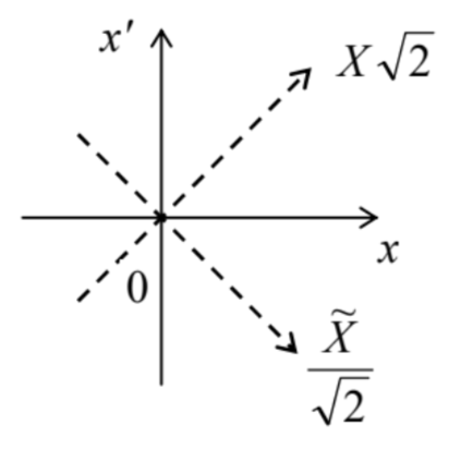
Unfortunately, besides the trivial case (30) of coinciding arguments, it is hard to give a straightforward interpretation of the density function in terms of the system’s measurements. This is a fundamental difficulty, which has been well explored in terms of the Wigner function (sometimes called the "Wigner-Ville distribution") \({ }^{18}\) defined as \[W(X, P) \equiv \frac{1}{2 \pi \hbar} \int w\left(X+\frac{\widetilde{X}}{2}, X-\frac{\widetilde{X}}{2}\right) \exp \left\{-\frac{i P \widetilde{X}}{\hbar}\right\} d \widetilde{X}\] From the mathematical standpoint, this is just the Fourier transform of the density matrix in one of two new coordinates defined by the following relations (see Fig. 2): \[X \equiv \frac{x+x^{\prime}}{2}, \quad \widetilde{X} \equiv x-x^{\prime}, \quad \text { so that } x \equiv X+\frac{\widetilde{X}}{2}, \quad x^{\prime} \equiv X-\frac{\widetilde{X}}{2} .\] Physically, the new argument \(X\) may be interpreted as the average position of the particle during the time interval \(\left(t-t^{\prime}\right)\), while \(\widetilde{X}\), as the distance passed by it during that time interval, so that \(P\) characterizes the momentum of the particle during that motion. As a result, the Wigner function is a mathematical construct intended to characterize the system’s probability distribution simultaneously in the coordinate and the momentum space - for 1D systems, on the phase plane \([X, P]\), which we had discussed earlier - see Fig. 5.8. Let us see how fruitful this intention is.

Fig. 7.2. The coordinates \(X\) and \(\tilde{X}\) employed in the WeylWigner transform (50). They differ from the coordinates obtained by the rotation of the reference frame by the angle \(\pi / 4\) only by factors \(\sqrt{2}\) and \(1 / \sqrt{2}\), describing scale stretch.

First of all, we may write the Fourier transform reciprocal to Eq. (50): \[w\left(X+\frac{\tilde{X}}{2}, X-\frac{\tilde{X}}{2}\right)=\int W(X, P) \exp \left\{\frac{i P \widetilde{X}}{\hbar}\right\} d P \text {. }\] For the particular case \(\widetilde{X}=0\), this relation yields \[w(X) \equiv w(X, X)=\int W(X, P) d P .\] Hence the integral of the Wigner function over the momentum \(P\) gives the probability density to find the system at point \(X\) - just as it does for a classical distribution function \(w_{\mathrm{cl}}(X, P) .{ }^{19}\)

Next, the Wigner function has the similar property for integration over \(X\). To prove this fact, we may first introduce the momentum representation of the density matrix, in full analogy with its coordinate representation (27): \[w\left(p, p^{\prime}\right) \equiv\left\langle p|\hat{w}| p^{\prime}\right\rangle .\] Inserting, as usual, two identity operators, in the form given by Eq. (4.252), into the right-hand side of this equality, we get the following relation between the momentum and coordinate representations: \[w\left(p, p^{\prime}\right)=\iint d x d x^{\prime}\langle p \mid x\rangle\left\langle x|\hat{w}| x^{\prime}\right\rangle\left\langle x^{\prime} \mid p^{\prime}\right\rangle=\frac{1}{2 \pi \hbar} \iint d x d x^{\prime} \exp \left\{-\frac{i p x}{\hbar}\right\} w\left(x, x^{\prime}\right) \exp \left\{+\frac{i p^{\prime} x^{\prime}}{\hbar}\right\} .\] This is of course nothing else than the unitary transform of an operator from the \(x\)-basis to the \(p\)-basis, similar to the first form of Eq. (4.272). For coinciding arguments, \(p=p^{\prime}\), Eq. (55) is reduced to \[w(p) \equiv w(p, p)=\frac{1}{2 \pi \hbar} \iint d x d x^{\prime} w\left(x, x^{\prime}\right) \exp \left\{-\frac{i p\left(x-x^{\prime}\right)}{\hbar}\right\} .\] Now using Eq. (29) and then Eq. (4.265), this function may be represented as \[w(p)=\frac{1}{2 \pi \hbar} \sum_{j} W_{j} \iint d x d x^{\prime} \psi_{j}(x) \psi_{j}^{*}(x) \exp \left\{-\frac{i p\left(x-x^{\prime}\right)}{\hbar}\right\}=\sum_{j} W_{j} \varphi_{j}(p) \varphi_{j}^{*}(p),\] and hence interpreted as the probability density of the particle’s momentum at value \(p\). Now, in the variables (51), Eq. (56) has the form

\[w(p)=\frac{1}{2 \pi \hbar} \iint w\left(X+\frac{\widetilde{X}}{2}, X-\frac{\widetilde{X}}{2}\right) \exp \left\{-\frac{i p \widetilde{X}}{\hbar}\right\} d \widetilde{X} d X .\] Comparing this equality with the definition (50) of the Wigner function, we see that \[w(P)=\int W(X, P) d X .\] Thus, according to Eqs. (53) and (59), the integrals of the Wigner function over either the coordinate or momentum give the probability densities to find the system at a certain value of the counterpart variable. This is of course the main requirement to any quantum-mechanical candidate for the best analog of the classical probability density, \(w_{\mathrm{cl}}(X, P)\).

Let us see at how does the Wigner function look for the simplest systems at thermodynamic equilibrium. For a free 1D particle, we can use Eq. (34), ignoring for simplicity the normalization issues: \[W(X, P) \propto \int_{-\infty}^{+\infty} \exp \left\{-\frac{m k_{\mathrm{B}} T \widetilde{X}^{2}}{2 \hbar^{2}}\right\} \exp \left\{-\frac{i P \widetilde{X}}{\hbar}\right\} d \widetilde{X} .\] The usual Gaussian integration yields: \[W(X, P)=\text { const } \times \exp \left\{-\frac{P^{2}}{2 m k_{\mathrm{B}} T}\right\} .\] We see that the function is independent of \(X\) (as it should be for this translational-invariant system), and coincides with the Gibbs distribution (24). We could get the same result directly from classical statistics. This is natural because as we know from Sec. 2.2, the free motion is essentially not quantized - at least in terms of its energy and momentum.

Now let us consider a substantially quantum system, the harmonic oscillator. Plugging Eq. (44) into Eq. (50), for that system in thermal equilibrium it is easy to show (and hence is left for reader’s exercise) that the Wigner function is also Gaussian, now in both its arguments: \[W(X, P)=\text { const } \times \exp \left\{-C\left[\frac{m \omega_{0}^{2} X^{2}}{2}+\frac{P^{2}}{2 m}\right]\right\},\] though the coefficient \(C\) is now different from \(1 / k_{\mathrm{B}} T\), and tends to that limit only at high temperatures, \(k_{\mathrm{B}} T \gg \hbar \omega_{0}\). Moreover, for a Glauber state, the Wigner function also gives a very plausible result \(-\mathrm{a}\) Gaussian distribution similar to Eq. (62), but properly shifted from the origin to the central point of the state \(-\) see Sec. 5.5. \({ }^{20}\)

Unfortunately, for some other possible states of the harmonic oscillator, e.g., any pure Fock state with \(n>0\), the Wigner function takes negative values in some regions of the \([X, P]\) plane \(-\) see Fig. \(3 .{ }^{21}\) (Such plots were the basis of my, admittedly very imperfect, classical images of the Fock states in Fig. 5.8.)

Fig. 7.3. The Wigner functions \(W(X, P)\) of a harmonic oscillator, in a few of its stationary (Fock) states \(n\) : (a) \(n=0\), (b) \(n=1\); (c) \(n=5\). Graphics by J. S. Lundeen; adapted from http://en.Wikipedia.org/wiki/Wigner function as a public-domain material.

The same is true for most other quantum systems and their states. Indeed, this fact could be predicted just by looking at the definition (50) applied to a pure quantum state, in which the density function may be factored - see Eq. (31): \[W(X, P)=\frac{1}{2 \pi \hbar} \int \psi\left(X+\frac{\tilde{X}}{2}\right) \psi^{*}\left(X-\frac{\tilde{X}}{2}\right) \exp \left\{-\frac{i P \tilde{X}}{\hbar}\right\} d \widetilde{X} .\] Changing the argument \(P\) (say, at fixed \(X\) ), we are essentially changing the spatial "frequency" (wave number) of the wavefunction product’s Fourier component we are calculating, and we know that their Fourier images typically change sign as the frequency is changed. Hence the wavefunctions should have some high-symmetry properties to avoid this effect. Indeed, the Gaussian functions (describing, for example, the Glauber states, and in their particular case, the ground state of the harmonic oscillator) have such symmetry, but many other functions do not.

Hence if the Wigner function was taken seriously as the quantum-mechanical analog of the classical probability density \(w_{\mathrm{cl}}(X, P)\), we would need to interpret the negative probability of finding the particle in certain elementary intervals \(d X d P\) - which is hard to do. However, the function is still used for a semi-quantitative interpretation of mixed states of quantum systems.

---

\({ }^{13}\) For now, I will focus on a fixed time instant (say, \(t=0\) ), and hence write \(\psi(x)\) instead of \(\Psi(x, t)\).

\({ }^{14}\) This fact is the origin of the density matrix’s name.

\({ }^{15}\) Due to the delta-normalization of the eigenfunction, the density matrix (34) for the free particle (and any system with a continuous eigenvalue spectrum) is normalized as \[\int_{-\infty}^{+\infty} w\left(x, x^{\prime}\right) Z d x^{\prime}=\int_{-\infty}^{+\infty} w\left(x, x^{\prime}\right) Z d x=1 \text {. }\]

\({ }^{16}\) I will have no time to discuss this technique and have to refer the interested reader to special literature. Probably, the most famous text of that field is A. Abrikosov, L. Gor’kov, and I. Dzyaloshinski, Methods of Quantum Field Theory in Statistical Physics, Prentice-Hall, 1963. (Later reprintings are available from Dover.)

17 I have to confess that this notation is imperfect, because strictly speaking, \(w\left(x, x^{\prime}\right)\) and \(w(x)\) are different functions, and so are the functions \(w\left(p, p^{\prime}\right)\) and \(w(p)\) used below. In the perfect world, I would use different letters for them all, but I desperately want to stay with " \(w\) " for all the probability densities, and there are not so many good fonts for this letter. Let me hope that the difference between these functions is clear from their arguments and the context.

\({ }^{18}\) It was introduced in 1932 by Eugene Wigner on the basis of a general (Weyl-Wigner) transform suggested by Hermann Weyl in 1927 and re-derived in 1948 by Jean Ville on a different mathematical basis.

\({ }^{19}\) Such function, used to express the probability \(d W\) to find the system in a small area of the phase plane as \(d W=w_{\mathrm{cl}}(X, P) d X d P\), is a major notion of the (1D) classical statistics - see, e.g., SM Sec. 2.1.

\({ }^{20}\) Please note that in the notation of Sec. 5.5, the capital letters \(X\) and \(P\) mean not the arguments of the Wigner function, but the Cartesian coordinates of the central point (5.102), i.e. the classical complex amplitude of the oscillations.

\({ }^{21}\) Spectacular experimental measurements of this function (for \(n=0\) and \(n=1\) ) were carried out recently by E. Bimbard et al., Phys. Rev. Lett. 112, 033601 (2014).