7.6: Density Matrix Approach

The main alternative approach to the dynamics of open quantum systems, which is essentially a generalization of the one discussed in Sec. 2, is to extract the final results of interest from the dynamics of the density operator of our system \(s\). Let us discuss this approach in detail. \({ }^{54}\)

We already know that the density matrix allows the calculation of the expectation value of any observable of the system \(s\) - see Eq. (5). However, our initial recipe (6) for the density matrix element calculation, which requires the knowledge of the exact state (2) of the whole Universe, is not too practicable, while the von Neumann equation (66) for the density matrix evolution is limited to cases in which probabilities \(W_{j}\) of the system states are fixed - thus excluding such important effects as the energy relaxation. However, such effects may be analyzed using a different assumption - that the system of interest interacts only with a local environment that is very close to its thermally-equilibrium state described, in the stationary-state basis, by a diagonal density matrix with the elements (24).

This calculation is facilitated by the following general observation. Let us number the basis states of the full local system (the system of our interest plus its local environment) by \(l\), and use Eq. (5) to write \[\langle A\rangle=\operatorname{Tr}\left(\hat{A} \hat{w}_{l}\right) \equiv \sum_{l, l^{\prime}} A_{l l^{\prime}} w_{l l}=\sum_{l, l^{\prime}}\left\langle l|\hat{A}| l^{\prime}\right\rangle\left\langle l^{\prime}\left|\hat{w}_{l}\right| l\right\rangle,\] where \(\hat{w}_{l}\) is the density operator of this local system. At a weak interaction between the system \(s\) and the local environment \(e\), their states reside in different Hilbert spaces, so that we can write \[|l\rangle=\left|s_{j}\right\rangle \otimes\left|e_{k}\right\rangle,\] and if the observable \(A\) depends only on the coordinates of the system \(s\) of our interest, we may reduce Eq. (157) to the form similar to Eq. (5): \[\begin{aligned} \langle A\rangle &=\sum_{j, j^{\prime}, k, k^{\prime}}\left\langle e_{k}\left|\otimes\left\langle s_{j}|\hat{A}| s_{j^{\prime}}\right\rangle \otimes\right| e_{k^{\prime}}\right\rangle\left\langle e_{k^{\prime}}\left|\otimes\left\langle s_{j^{\prime}}\left|\hat{w}_{l}\right| s_{j}\right\rangle \otimes\right| e_{k}\right\rangle \\ &=\sum_{j, j^{\prime}} A_{i j^{\prime}}\left\langle s_{j^{\prime}}\left(\sum_{k} \otimes\left\langle e_{k}\left|\hat{w}_{l}\right| e_{k}\right\rangle \otimes\right) \mid s_{j}\right\rangle=\operatorname{Tr}_{j}(\hat{A} \hat{w}), \end{aligned}\] where \[\hat{w} \equiv \sum_{k}\left\langle e_{k}\left|\hat{w}_{l}\right| e_{k}\right\rangle=\operatorname{Tr}_{k} \hat{w}_{l},\] showing how exactly the density operator \(\hat{w}\) of the system \(s\) may be calculated from \(\hat{w}_{l}\).

Now comes the key physical assumption of this approach: since we may select the local environment \(e\) to be much larger than the system \(s\) of our interest, we may consider the composite system \(l\) as a Hamiltonian one, with time-independent probabilities of its stationary states, so that for the description of the evolution in time of \(i t s\) full density operator \(\hat{w}_{l}\) (again, in contrast to that, \(\hat{w}\), of the system of our interest) we may use the von Neumann equation (66). Partitioning its right-hand side in accordance with Eq. (68), we get: \[i \hbar \dot{\hat{w}}_{l}=\left[\hat{H}_{s}, \hat{w}_{l}\right]+\left[\hat{H}_{e}, \hat{w}_{l}\right]+\left[\hat{H}_{\mathrm{int}}, \hat{w}_{l}\right] .\] The next step is to use the perturbation theory to solve this equation in the lowest order in \(\hat{H}_{\text {int }}\), which would yield, for the evolution of \(w\), a non-vanishing contribution due to the interaction. For that, Eq. (161) is not very convenient, because its right-hand side contains two other terms, of a much larger scale than the interaction Hamiltonian. To mitigate this technical difficulty, the interaction picture that was discussed at the end of \(\mathrm{Sec} .4 .6\), is very natural. (It is not necessary though, and I will use this picture mostly as an exercise of its application - unfortunately, the only example I can afford in this course.)

As a reminder, in that picture (whose entities will be marked with index "I", with the unmarked operators assumed to be in the Schrödinger picture), both the operators and the state vectors (and hence the density operator) depend on time. However, the time evolution of the operator of any observable \(A\) is described by an equation similar to Eq. (67), but with the unperturbed part of the Hamiltonian only - see Eq. (4.214). In model (68), this means \[i \hbar \dot{\hat{A}}_{\mathrm{I}}=\left[\hat{A}_{\mathrm{I}}, \hat{H}_{0}\right] .\] where the unperturbed Hamiltonian consists of two parts defined in different Hilbert spaces: \[\hat{H}_{0} \equiv \hat{H}_{s}+\hat{H}_{e} \text {. }\] On the other hand, the state vector’s dynamics is governed by the interaction evolution operator \(\hat{u}_{1}\) that obeys Eqs. (4.215). Since this equation, using the interaction-picture Hamiltonian (4.216), \[\hat{H}_{\mathrm{I}} \equiv \hat{u}_{0}^{\dagger} \hat{H}_{\mathrm{int}} \hat{u}_{0},\] is absolutely similar to the ordinary Schrödinger equation using the full Hamiltonian, we may repeat all arguments given at the beginning of \(\mathrm{Sec} .3\) to prove that the dynamics of the density operator in the interaction picture of a Hamiltonian system is governed by the following analog of the von Neumann equation (66): \[i \hbar \dot{\hat{w}}_{\mathrm{I}}=\left[\hat{H}_{\mathrm{I}}, \hat{w}_{\mathrm{I}}\right]\] where the index \(l\) is dropped for the notation simplicity. Since this equation is similar in structure (with the opposite sign) to the Heisenberg equation (67), we may use the solution Eq. (4.190) of the latter equation to write its analog: \[\hat{w}_{\mathrm{I}}(t)=\hat{u}_{\mathrm{I}}(t, 0) \hat{w}_{l}(0) \hat{u}_{\mathrm{I}}^{\dagger}(t, 0) .\] It is also straightforward to verify that in this picture, the expectation value of any observable \(A\) may be found from an expression similar to the basic Eq. (5): \[\langle A\rangle=\operatorname{Tr}\left(\hat{A}_{\mathrm{I}} \hat{w}_{\mathrm{I}}\right),\] showing again that the interaction and Schrödinger pictures give the same final results.

In the most frequent case of factorable interaction (90), \({ }^{55}\) Eq. (162) is simplified for both operators participating in that product \(-\) for each one in its own way. In particular, for \(\hat{A}=\hat{x}\), it yields

\[i \hbar \dot{\hat{x}}_{\mathrm{I}}=\left[\hat{x}_{1}, \hat{H}_{0}\right] \equiv\left[\hat{x}_{\mathrm{I}}, \hat{H}_{s}\right]+\left[\hat{x}_{\mathrm{I}}, \hat{H}_{e}\right] .\] Since the coordinate operator is defined in the Hilbert space of our system \(s\), it commutes with the Hamiltonian of the environment, so that we finally get \[i \hbar \dot{\hat{x}}_{\mathrm{I}}=\left[\hat{x}_{\mathrm{I}}, \hat{H}_{s}\right] \text {. }\] On the other hand, if \(\hat{A}=\hat{F}\), this operator is defined in the Hilbert space of the environment, and commutes with the Hamiltonian of the unperturbed system \(s\). As a result, we get \[i \hbar \dot{\hat{F}}_{\mathrm{I}}=\left[\hat{F}_{\mathrm{I}}, \hat{H}_{e}\right] \text {. }\] This means that with our time-independent unperturbed Hamiltonians, \(\hat{H}_{s}\) and \(\hat{H}_{e}\), the time evolution of the interaction-picture operators is rather simple. In particular, the analogy between Eq. \((170)\) and Eq. (93) allows us to immediately write the following analog of Eq. (94): \[\hat{F}_{\mathrm{I}}(t)=\exp \left\{+\frac{i}{\hbar} \hat{H}_{e} t\right\} \hat{F}(0) \exp \left\{-\frac{i}{\hbar} \hat{H}_{e} t\right\} \text {, }\] so that in the stationary-state basis \(n\) of the environment, \[\left(\hat{F}_{\mathrm{I}}\right)_{n n^{\prime}}(t)=\exp \left\{+\frac{i}{\hbar} E_{n} t\right\} F_{n n^{\prime}}(0) \exp \left\{-\frac{i}{\hbar} E_{n^{\prime}} t\right\} \equiv F_{n n^{\prime}}(0) \exp \left\{-i \frac{E_{n}-E_{n^{\prime}}}{\hbar} t\right\},\] and similarly (but in the basis of the stationary states of system \(s\) ) for operator \(\hat{x}\). As a result, the righthand side of Eq. (164) may be also factored: \[\begin{aligned} \hat{H}_{\mathrm{I}}(t) & \equiv \hat{u}_{0}^{\dagger}(t, 0) \hat{H}_{\mathrm{int}} \hat{u}_{0}(t, 0)=\exp \left\{\frac{i}{\hbar}\left(\hat{H}_{s}+\hat{H}_{e}\right) t\right\}(-\hat{x} \hat{F}) \exp \left\{-\frac{i}{\hbar}\left(\hat{H}_{s}+\hat{H}_{e}\right) t\right\} \\ &=-\left(\exp \left\{+\frac{i}{\hbar} \hat{H}_{s} t\right\} \hat{x} \exp \left\{-\frac{i}{\hbar} \hat{H}_{s} t\right\}\right)\left(\exp \left\{+\frac{i}{\hbar} \hat{H}_{e} t\right\} \hat{F}(0) \exp \left\{-\frac{i}{\hbar} \hat{H}_{e} t\right\}\right) \equiv-\hat{x}_{I}(t) \hat{F}_{\mathrm{I}}(t) . \end{aligned}\] So, the transfer to the interaction picture has taken some time, but now it enables a smooth ride. \({ }^{56}\) Indeed, just as in Sec. 4, we may rewrite Eq. (165) in the integral form: \[\hat{w}_{\mathrm{I}}(t)=\frac{1}{i \hbar} \int_{-\infty}^{t}\left[\hat{H}_{\mathrm{I}}\left(t^{\prime}\right), \hat{w}_{\mathrm{I}}\left(t^{\prime}\right)\right] d t^{\prime} ;\] plugging this result into the right-hand side of Eq. (165), we get \[\dot{\hat{w}}_{\mathrm{I}}(t)=-\frac{1}{\hbar^{2}} \int_{-\infty}^{t}\left[\hat{H}_{\mathrm{I}}(t),\left[\hat{H}_{\mathrm{I}}\left(t^{\prime}\right), \hat{w}_{\mathrm{I}}\left(t^{\prime}\right)\right]\right] d t^{\prime}=-\frac{1}{\hbar^{2}} \int_{-\infty}^{t}\left[\hat{x}(t) \hat{F}(t),\left[\hat{x}\left(t^{\prime}\right) \hat{F}\left(t^{\prime}\right), \hat{w}_{\mathrm{I}}\left(t^{\prime}\right)\right]\right] d t^{\prime},\] where, for the notation’s brevity, from this point on I will strip the operators \(\hat{x}\) and \(\hat{F}\) of their index "I". (I hope their time dependence indicates the interaction picture clearly enough.)

So far, this equation is exact (and cannot be solved analytically), but this is a good time to notice that even if we approximate the density operator on its right-hand side by its unperturbed, factorable "value" (corresponding to no interaction between the system \(s\) and its thermally-equilibrium environment \(e\) ), \({ }^{57}\) \[\hat{w}_{1}\left(t^{\prime}\right) \rightarrow \hat{w}\left(t^{\prime}\right) \hat{w}_{e}, \quad \text { with }\left\langle e_{n}\left|\hat{w}_{e}\right| e_{n^{\prime}}\right\rangle=W_{n} \delta_{n n^{\prime}}\] where \(e_{n}\) are the stationary states of the environment and \(W_{n}\) are the Gibbs probabilities (24), Eq. (175) still describes nontrivial time evolution of the density operator. This is exactly the first non-vanishing approximation (in the weak interaction) we have been looking for. Now using Eq. (160), we find the equation of evolution of the density operator of the system of our interest: \[\dot{\hat{w}}(t)=-\frac{1}{\hbar^{2}} \int_{-\infty}^{t} \operatorname{Tr}_{n}\left[\hat{x}(t) \hat{F}(t),\left[\hat{x}\left(t^{\prime}\right) \hat{F}\left(t^{\prime}\right), \hat{w}\left(t^{\prime}\right) \hat{w}_{e}\right]\right] d t^{\prime},\] where the trace is over the stationary states of the environment. To spell out the right-hand side of Eq. (177), note again that the coordinate and force operators commute with each other (but not with themselves at different time moments!) and hence may be swapped at will, so that we may write \[\begin{aligned} \operatorname{Tr}_{n}[\ldots,[\ldots, \ldots]]=& \hat{x}(t) \hat{x}\left(t^{\prime}\right) \hat{w}\left(t^{\prime}\right) \operatorname{Tr}_{n}\left[\hat{F}(t) \hat{F}\left(t^{\prime}\right) \hat{w}_{e}\right]-\hat{x}(t) \hat{w}\left(t^{\prime}\right) \hat{x}\left(t^{\prime}\right) \operatorname{Tr}_{n}\left[\hat{F}(t) \hat{w}_{e} \hat{F}\left(t^{\prime}\right)\right] \\ &-\hat{x}\left(t^{\prime}\right) \hat{w}\left(t^{\prime}\right) \hat{x}(t) \operatorname{Tr}_{n}\left[\hat{F}\left(t^{\prime}\right) \hat{w}_{e} \hat{F}(t)\right]+\hat{w}\left(t^{\prime}\right) \hat{x}\left(t^{\prime}\right) \hat{x}(t) \operatorname{Tr}_{n}\left[\hat{w}_{e} \hat{F}\left(t^{\prime}\right) \hat{F}(t)\right] \\ =& \hat{x}(t) \hat{x}\left(t^{\prime}\right) \hat{w}\left(t^{\prime}\right) \sum_{n, n^{\prime}} F_{n n^{\prime}}(t) F_{n^{\prime} n}\left(t^{\prime}\right) W_{n}-\hat{x}(t) \hat{w}\left(t^{\prime}\right) \hat{x}\left(t^{\prime}\right) \sum_{n, n^{\prime}} F_{n n^{\prime}}(t) W_{n^{\prime}} F_{n^{\prime} n}\left(t^{\prime}\right) \\ &-\hat{x}\left(t^{\prime}\right) \hat{w}\left(t^{\prime}\right) \hat{x}(t) \sum_{n, n^{\prime}} F_{n n^{\prime}}\left(t^{\prime}\right) W_{n^{\prime}} F_{n^{\prime} n}(t)+\hat{w}\left(t^{\prime}\right) \hat{x}\left(t^{\prime}\right) \hat{x}(t) \sum_{n, n^{\prime}} W_{n} F_{n n^{\prime}}\left(t^{\prime}\right) F_{n^{\prime} n}(t) . \end{aligned}\] Since the summation over both indices \(n\) and \(n\) ’ in this expression is over the same energy level set (of all stationary states of the environment), we may swap these indices in any of the sums. Doing this only in the terms including the factors \(W_{n}\), we turn them into \(W_{n}\), so that this factor becomes common: \[\begin{aligned} \operatorname{Tr}_{n}[\ldots,[\ldots, \ldots]]=\sum_{n, n^{\prime}} W_{n}\left[\hat{x}(t) \hat{x}\left(t^{\prime}\right) \hat{w}\left(t^{\prime}\right) F_{n n^{\prime}}(t) F_{n^{\prime} n}\left(t^{\prime}\right)-\hat{x}(t) \hat{w}\left(t^{\prime}\right) \hat{x}\left(t^{\prime}\right) F_{n^{\prime} n}(t) F_{n n^{\prime}}\left(t^{\prime}\right)\right.&\left.-\hat{x}\left(t^{\prime}\right) \hat{w} \hat{x}(t) F_{n^{\prime} n}\left(t^{\prime}\right) F_{n n^{\prime}}(t)+\hat{w} \hat{x}\left(t^{\prime}\right) \hat{x}(t) F_{n n^{\prime}}\left(t^{\prime}\right) F_{n^{\prime} n}(t)\right] . \end{aligned}\] Now using Eq. (172), we get \[\begin{aligned} \operatorname{Tr}_{n}[\ldots,[\ldots, \ldots]] &=\sum_{n, n^{\prime}} W_{n}\left|F_{n n^{\prime}}\right|^{2} \times\left[\begin{array}{l} \hat{x}(t) \hat{x}\left(t^{\prime}\right) \hat{w}\left(t^{\prime}\right) \exp \left\{+\frac{i \widetilde{E}\left(t-t^{\prime}\right)}{\hbar}\right\}-\hat{x}(t) \hat{w}\left(t^{\prime}\right) \hat{x}\left(t^{\prime}\right) \exp \left\{-\frac{i \widetilde{E}\left(t-t^{\prime}\right)}{\hbar}\right\} \\ \left.-\hat{x}\left(t^{\prime}\right) \hat{w}\left(t^{\prime}\right) \hat{x}(t) \exp \left\{+\frac{i \widetilde{E}\left(t-t^{\prime}\right)}{\hbar}\right\}+\hat{w}\left(t^{\prime}\right) \hat{x}\left(t^{\prime}\right) \hat{x}(t) \exp \left\{-\frac{i \widetilde{E}\left(t-t^{\prime}\right)}{\hbar}\right\}\right] \end{array}\right.\\ & \equiv \sum_{n, n^{\prime}} W_{n}\left|F_{n n^{\prime}}\right|^{2} \cos \frac{\widetilde{E}\left(t-t^{\prime}\right)}{\hbar}\left[\hat{x}(t),\left[\hat{x}\left(t^{\prime}\right), \hat{w}\left(t^{\prime}\right)\right]\right]+i \sum_{n, n^{\prime}} W_{n}\left|F_{n n^{\prime}}\right|^{2} \sin \frac{\widetilde{E}\left(t-t^{\prime}\right)}{\hbar}\left[\hat{x}(t),\left\{\hat{x}\left(t^{\prime}\right), \hat{w}\left(t^{\prime}\right)\right\}\right] \end{aligned}\] Comparing the two double sums participating in this expression with Eqs. (108) and (111), we see that they are nothing else than, respectively, the symmetrized correlation function and the temporal Green’s function (multiplied by \(\hbar / 2\) ) of the time-difference argument \(\tau=t-t^{\prime} \geq 0\). As the result, Eq. (177) takes a compact form: \[\dot{\hat{w}}(t)=-\frac{1}{\hbar^{2}} \int_{-\infty}^{t} K_{F}\left(t-t^{\prime}\right)\left[\hat{x}(t),\left[\hat{x}\left(t^{\prime}\right), \hat{w}\left(t^{\prime}\right)\right]\right] d t^{\prime}-\frac{i}{2 \hbar} \int_{-\infty}^{t} G\left(t-t^{\prime}\right)\left[\hat{x}(t),\left\{\hat{x}\left(t^{\prime}\right), \hat{w}\left(t^{\prime}\right)\right\}\right] d t^{\prime}\] Let me hope that the readers (especially the ones who have braved through this derivation) enjoy this beautiful result as much as I do. It gives an equation for the time evolution of the density operator of the system of our interest \((s)\), with the effects of its environment represented only by two real, \(c\)-number functions of \(\tau\) : one \(\left(K_{F}\right)\) describing the fluctuation force exerted by the environment, and the other one \((G)\) representing its ensemble-averaged environment’s response to the system’s evolution. And most spectacularly, these are exactly the same functions that participate in the alternative, HeisenbergLangevin approach to the problem, and hence related to each other by the fluctuation-dissipation theorem (134).

After a short celebration, let us acknowledge that Eq. (181) is still an integro-differential equation, and needs to be solved together with Eq. (169) for the system coordinate’s evolution. Such equations do not allow explicit analytical solutions, besides a few very simple (and not very interesting) cases. For most applications, further simplifications should be made. One of them is based on the fact (which was already discussed in Sec. 3) that both environmental functions participating in Eq. (181) tend to zero when their argument \(\tau\) becomes much larger than the environment’s correlation time \(\tau_{\mathrm{c}}\), independent of the system-to-environment coupling strength. If the coupling is sufficiently weak, the time scales \(T_{n n}\) ’ of the evolution of the density matrix elements, following from Eq. (181), are much longer than this correlation time, and also the characteristic time scale of the coordinate operator’s evolution. In this limit, all arguments \(t^{\prime}\) of the density operator, giving substantial contributions to the right-hand side of Eq. (181), are so close to \(t\) that it does not matter whether its argument is \(t\) ’ or just \(t\). This simplification, \(w\left(t^{\prime}\right) \approx w(t)\), is known as the Markov approximation. \({ }^{58}\)However, this approximation alone is still insufficient for finding the general solution of Eq. (181). Substantial further progress is possible in two important cases. The most important of them is when the intrinsic Hamiltonian \(\hat{H}_{s}\) of the system \(s\) of our of interest does not depend on time explicitly and has a discrete eigenenergy spectrum \(E_{n}{ }^{59}\) with well-separated levels: \[\left|E_{n}-E_{n^{\prime}}\right|>>\frac{\hbar}{T_{n n^{\prime}}} \text {. }\] Let us see what does this condition yield for Eq. (181), rewritten for the matrix elements in the stationary state basis, in the Markov approximation: \[\dot{w}_{n n^{\prime}}=-\frac{1}{\hbar^{2}} \int_{-\infty}^{t} K_{F}\left(t-t^{\prime}\right)\left[\hat{x}(t),\left[\hat{x}\left(t^{\prime}\right), \hat{w}\right]\right]_{n n^{\prime}} d t^{\prime}-\frac{i}{2 \hbar} \int_{-\infty}^{t} G\left(t-t^{\prime}\right)\left[\hat{x}(t),\left\{\hat{x}\left(t^{\prime}\right), \hat{w}\right\}\right]_{n n^{\prime}} d t^{\prime} .\] After spelling out the commutators, the right-hand side of this expression includes four operator products, which differ "only" by the operator order. Let us first have a look at one of these products, \[\left[\hat{x}(t) \hat{x}\left(t^{\prime}\right) \hat{w}\right]_{n n^{\prime}} \equiv \sum_{m, m^{\prime}} x_{n m}(t) x_{m m^{\prime}}\left(t^{\prime}\right) w_{m^{\prime} n^{\prime}},\] where the indices \(m\) and \(m\) ’ run over the same set of stationary states of the system \(s\) of our interest as the indices \(n\) and \(n\) ’. According to Eq. (169) with a time-independent \(H_{s}\), the matrix elements \(x_{n n^{\prime}}\) ’ (in the stationary state basis) oscillate in time as \(\exp \left\{i \omega_{n n} t\right\}\), so that \[\left[\hat{x}(t) \hat{x}\left(t^{\prime}\right) \hat{w}\right]_{m n^{\prime}}=\sum_{m, m^{\prime}} x_{n m} x_{m m^{\prime}}, \exp \left\{i\left(\omega_{n m} t+\omega_{m m^{\prime}} t^{\prime}\right)\right\} w_{m^{\prime} n^{\prime}},\] where on the right-hand side, the coordinate matrix elements are in the Schrödinger picture, and the usual notation \((6.85)\) is used for the quantum transition frequencies: \[\hbar \omega_{n n^{\prime}} \equiv E_{n}-E_{n^{\prime}} .\] According to the condition (182), frequencies \(\omega_{n n^{\prime}}\) with \(n \neq n^{\prime}\) are much higher than the speed of evolution of the density matrix elements (in the interaction picture!) - on both the left-hand and righthand sides of Eq. (183). Hence, on the right-hand side of Eq. (183), we may keep only the terms that do not oscillate with these frequencies \(\omega_{n n}\), because rapidly-oscillating terms would give negligible contributions to the density matrix dynamics. \({ }^{60}\) For that, in the double sum (185) we should save only the terms proportional to the difference \(\left(t-t^{\prime}\right)\) because they will give (after the integration over \(t^{\prime}\) ) a slowly changing contribution to the right-hand side. \({ }^{61}\) These terms should have \(\omega_{n m}+\omega_{m m}{ }^{\prime}=0\), i.e. \(\left(E_{n}-\right.\) \(\left.E_{m}\right)+\left(E_{m}-E_{m^{\prime}}\right) \equiv E_{n}-E_{m^{\prime}}=0\). For a non-degenerate energy spectrum, this requirement means \(m^{\prime}=n\); as a result, the double sum is reduced to a single one: \[\left[\hat{x}(t) \hat{x}\left(t^{\prime}\right) \hat{w}\right]_{n n^{\prime}} \approx w_{n n^{\prime}} \sum_{m} x_{n m} x_{m n} \exp \left\{i \omega_{n m}\left(t-t^{\prime}\right)\right\} \equiv w_{n n^{\prime}} \sum_{m}\left|x_{n m}\right|^{2} \exp \left\{i \omega_{n m}\left(t-t^{\prime}\right)\right\}\] Another product, \(\left[\hat{w} \hat{x}\left(t^{\prime}\right) \hat{x}(t)\right]_{n n^{\prime}}\), which appears on the right-hand side of Eq. (183), may be simplified absolutely similarly, giving \[\left[\hat{w} \hat{x}\left(t^{\prime}\right) \hat{x}(t)\right]_{n n^{\prime}} \approx \sum_{m}\left|x_{n^{\prime} m}\right|^{2} \exp \left\{i \omega_{n^{\prime} m}\left(t^{\prime}-t\right)\right\} w_{n n^{\prime}} .\] These expressions hold whether \(n\) and \(n\) ’ are equal or not. The situation is different for two other products on the right-hand side of Eq. (183), with \(w\) sandwiched between \(x(t)\) and \(x\left(t^{\prime}\right)\). For example, \[\left[\hat{x}(t) \hat{w} \hat{x}\left(t^{\prime}\right)\right]_{n n^{\prime}}=\sum_{m, m^{\prime}} x_{n m}(t) w_{m m^{\prime}} x_{m^{\prime} n^{\prime}}\left(t^{\prime}\right)=\sum_{m, m^{\prime}} x_{n m} w_{m m^{\prime}} x_{m^{\prime} n^{\prime}} \exp \left\{i\left(\omega_{n m} t+\omega_{m^{\prime} n^{\prime}} t^{\prime}\right)\right\} .\] For this term, the same requirement of having a fast oscillating function of \(\left(t-t^{\prime}\right)\) only, yields a different condition: \(\omega_{n m}+\omega_{m^{\prime} n^{\prime}}=0\), i.e. \[\left(E_{n}-E_{m}\right)+\left(E_{m^{\prime}}-E_{n^{\prime}}\right)=0 .\] Here the double sum’s reduction is possible only if we make an additional assumption that all interlevel energy distances are unique, i.e. our system of interest has no equidistant levels (such as in the harmonic oscillator). For the diagonal elements \(\left(n=n^{\prime}\right)\), the RWA requirement is reduced to \(m=m\) ’, giving sums over all diagonal elements of the density matrix: \[\left[\hat{x}(t) \hat{w} \hat{x}\left(t^{\prime}\right)\right]_{n n}=\sum_{m}\left|x_{n m}\right|^{2} \exp \left\{i \omega_{n m}\left(t-t^{\prime}\right)\right\} w_{m m} .\] (Another similar term, \(\left[\hat{x}\left(t^{\prime}\right) \hat{w} \hat{x}(t)\right]_{n n}\), is just a complex conjugate of (191).) However, for off-diagonal matrix elements \(\left(n \neq n^{\prime}\right)\), the situation is different: Eq. (190) may be satisfied only if \(m=n\) and also \(m\) ’ \(=n^{\prime}\), so that the double sum is reduced to just one, non-oscillating term: \[\left[\hat{x}(t) \hat{w} \hat{x}\left(t^{\prime}\right)\right]_{n n^{\prime}}=x_{n n} w_{n n^{\prime}} x_{n^{\prime} n^{\prime}}, \text { for } n \neq n^{\prime} .\] The second similar term, \(\left[\hat{x}\left(t^{\prime}\right) \hat{w} \hat{x}(t)\right]_{n n}\), is exactly the same, so that in one of the integrals of Eq. (183), these terms add up, while in the second one, they cancel.

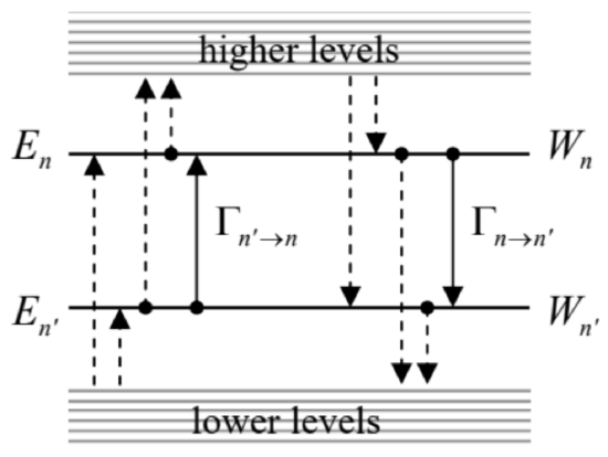
This is why the final equations of evolution look differently for diagonal and off-diagonal elements of the density matrix. For the former case \(\left(n=n^{\prime}\right)\), Eq. (183) is reduced to the so-called master equation \(^{62}\) relating diagonal elements \(w_{n n}\) of the density matrix, i.e. the energy level occupancies \(W_{n}:{ }^{63}\) \[\begin{aligned} \dot{W}_{n}=\sum_{m \neq n}\left|x_{n m}\right|^{2} \int_{0}^{\infty}[&-\frac{1}{\hbar^{2}} K_{F}(\tau)\left(W_{n}-W_{m}\right)\left(\exp \left\{i \omega_{n m} \tau\right\}+\exp \left\{-i \omega_{n m} \tau\right\}\right) \\ &\left.-\frac{i}{2 \hbar} G(\tau)\left(-W_{n}-W_{m}\right)\left(\exp \left\{i \omega_{n m} \tau\right\}-\exp \left\{-i \omega_{n m} \tau\right\}\right)\right] d \tau \end{aligned}\] where \(\tau \equiv t-t^{\prime}\). Changing the summation index notation from \(m\) to \(n\) ’, we may rewrite the master equation in its canonical form \[\dot{W}_{n}=\sum_{n^{\prime} \neq n}\left(\Gamma_{n^{\prime} \rightarrow n} W_{n^{\prime}}-\Gamma_{n \rightarrow n^{\prime}} W_{n}\right)\] where the coefficients \[\Gamma_{n^{\prime} \rightarrow n} \equiv\left|x_{n n^{\prime}}\right|^{2} \int_{0}^{\infty}\left[\frac{2}{\hbar^{2}} K_{F}(\tau) \cos \omega_{n n^{\prime}} \tau-\frac{1}{\hbar} G(\tau) \sin \omega_{n n^{\prime}} \tau\right] d t^{\prime},\] are called the interlevel transition rates. \({ }^{64}\) Eq. (194) has a very clear physical meaning of the level occupancy dynamics (i.e. the balance of the probability flows \(\Gamma W\) ) due to quantum transitions between the energy levels (see Fig. 7), in our current case caused by the interaction between the system of our interest and its environment.

Fig. 7.7. Probability flows in a discretespectrum system. Solid arrows: the exchange between the two energy levels, \(n\) and \(n^{\prime}\), described by one term in the master equation (194); dashed arrows: other transitions to/from these two levels.

The Fourier transforms (113) and (123) enable us to express the two integrals in Eq. (195) via, respectively, the symmetrized spectral density \(S_{F}(\omega)\) of environment force fluctuations and the imaginary part \(\chi^{\prime \prime}(\omega)\) of the generalized susceptibility, both at frequency \(\omega=\omega_{n n}\). After that we may use the fluctuation-dissipation theorem (134) to exclude the former function, getting finally \({ }^{65}\)

\(\begin{array}{T}\text { Transition } \\ \text { rates via } \\ \chi^{\prime \prime}(\omega)\end{array} \quad \Gamma_{n^{\prime} \rightarrow n}=\frac{1}{\hbar}\left|x_{n n^{\prime}}\right|^{2} \chi^{\prime \prime}\left(\omega_{n n^{\prime}}\right)\left(\operatorname{coth} \frac{\hbar \omega_{n n^{\prime}}}{2 k_{\mathrm{B}} T}-1\right) \equiv \frac{2}{\hbar}\left|x_{n n^{\prime}}\right|^{2} \frac{\chi^{\prime \prime}\left(\omega_{n n^{\prime}}\right)}{\exp \left\{\left(E_{n}-E_{n^{\prime}}\right) / k_{\mathrm{B}} T\right\}-1} .\)

Note that since the imaginary part \(\chi\) " of the generalized susceptibility is an odd function of frequency, Eq. (196) is in compliance with the Gibbs distribution for arbitrary temperature. Indeed, according to this equation, the ratio of the "up" and "down" rates for each pair of levels equals \[\frac{\Gamma_{n^{\prime} \rightarrow n}}{\Gamma_{n \rightarrow n^{\prime}}}=\frac{\chi^{\prime \prime}\left(\omega_{n n^{\prime}}\right)}{\exp \left\{\left(E_{n}-E_{n^{\prime}}\right) / k_{\mathrm{B}} T\right\}-1} / \frac{\chi^{\prime \prime}\left(\omega_{n^{\prime} n}\right)}{\exp \left\{\left(E_{n^{\prime}}-E_{n}\right) / k_{\mathrm{B}} T\right\}-1} \equiv \exp \left\{-\frac{E_{n}-E_{n^{\prime}}}{k_{\mathrm{B}} T}\right\}\] On the other hand, according to the Gibbs distribution (24), in thermal equilibrium the level populations should be in the same proportion. Hence, Eq. (196) complies with the so-called detailed balance equation, \[W_{n} \Gamma_{n \rightarrow n^{\prime}}=W_{n^{\prime}} \Gamma_{n^{\prime} \rightarrow n},\] valid in the equilibrium for each pair \(\left\{n, n^{\prime}\right\}\), so that all right-hand sides of all Eqs. (194), and hence the time derivatives of all \(W_{n}\) vanish - as they should. Thus, the stationary solution of the master equations indeed describes the thermal equilibrium correctly.

The system of master equations (194), frequently complemented by additional terms on their right-hand sides, describing interlevel transitions due to other factors (e.g., by an external ac force with a frequency close to one of \(\omega_{n n}\) ’), is the key starting point for practical analyses of many quantum systems, notably including optical quantum amplifiers and generators (lasers). It is important to remember that they are strictly valid only in the rotating-wave approximation, i.e. if Eq. (182) is well satisfied for all \(n\) and \(n\) ’ of substance.For a particular but very important case of a two-level system (with, say, \(E_{1}>E_{2}\) ), the rate \(\Gamma_{1 \rightarrow 2}\) may be interpreted (especially in the low-temperature limit \(k_{\mathrm{B}} T<<\hbar_{12}=E_{1}-E_{2}\), when \(\Gamma_{1 \rightarrow 2} \gg \Gamma_{2 \rightarrow 1}\) ) as the reciprocal characteristic time \(1 / T_{1} \equiv \Gamma_{1 \rightarrow 2}\) of the energy relaxation process that brings the diagonal elements of the density matrix to their thermally-equilibrium values (24). For the Ohmic dissipation described by Eqs. (137)-(138), Eq. (196) yields \[\frac{1}{T_{1}} \equiv \Gamma_{1 \rightarrow 2}=\frac{2}{\hbar^{2}}\left|x_{12}\right|^{2} \eta \times \begin{cases}\hbar \omega_{12}, & \text { for } k_{\mathrm{B}} T<<\hbar \omega_{12}, \\ k_{\mathrm{B}} T, & \text { for } \hbar \omega_{12}<<k_{\mathrm{B}} T .\end{cases}\] This relaxation time \(T_{1}\) should not be confused with the characteristic time \(T_{2}\) of the off-diagonal element decay, i.e. dephasing, which was already discussed in Sec. 3. In this context, let us see what do Eqs. (183) have to say about the dephasing rates. Taking into account our intermediate results (187)(192), and merging the non-oscillating components (with \(m=n\) and \(m=n^{\prime}\) ) of the sums Eq. (187) and (188) with the terms (192), which also do not oscillate in time, we get the following equation: 66 \[\begin{aligned} \dot{w}_{n n^{\prime}}=-&\left\{\begin{array}{l} \int_{0}^{\infty}\left[\frac{1}{\hbar^{2}} K_{F}(\tau)\left(\sum_{m \neq n}\left|x_{n m}\right|^{2} \exp \left\{i \omega_{n m} \tau\right\}+\sum_{m \neq n^{\prime}}\left|x_{n^{\prime} m}\right|^{2} \exp \left\{-i \omega_{n^{\prime} m} \tau\right\}+\left(x_{n n}-x_{n^{\prime \prime}{ }^{\prime}}\right)^{2}\right)\right. \\ & \left.\left.+\frac{i}{2 \hbar} G(\tau)\left(\sum_{m \neq n}\left|x_{n m}\right|^{2} \exp \left\{i \omega_{n m} \tau\right\}-\sum_{m \neq n^{\prime}}\left|x_{n^{\prime} m}\right|^{2} \exp \left\{-i \omega_{n^{\prime} m} \tau\right\}\right)\right] d \tau\right\} w_{n n^{\prime}}, \text { for } n \neq n^{\prime} . \end{array}\right. \end{aligned}\] In contrast with Eq. (194), the right-hand side of this equation includes both a real and an imaginary part, and hence it may be represented as \[\dot{w}_{n n^{\prime}}=-\left(1 / T_{n n^{\prime}}+i \Delta_{n n^{\prime}}\right) w_{n n^{\prime}},\] where both factors \(1 / T_{n n}\) ’ and \(\Delta_{n n}\) ’ are real. As Eq. (201) shows, the second term in the right-hand side of this equation causes slow oscillations of the matrix elements \(w_{n n}\), which, after returning to the Schrödinger picture, add just small corrections 67 to the unperturbed frequencies (186) of their oscillations, and are not important for most applications. More important is the first term, proportional to \[\frac{1}{T_{n n^{\prime}}}=\int_{0}^{\infty}\left[\frac{1}{\hbar^{2}} K_{F}(\tau)\left(\sum_{m \neq n}\left|x_{n m}\right|^{2} \cos \omega_{n m} \tau+\sum_{m \neq n^{\prime}}\left|x_{n^{\prime} m}\right|^{2} \cos \omega_{n^{\prime} m} \tau+\left(x_{n n}-x_{n^{\prime} n^{\prime}}\right)^{2}\right)\right.\] \[\left.-\frac{1}{2 \hbar} G(\tau)\left(\sum_{m \neq n}\left|x_{n m}\right|^{2} \sin \omega_{n m} \tau+\sum_{m \neq n^{\prime}}\left|x_{n^{\prime} m}\right|^{2} \sin \omega_{n^{\prime} m} \tau\right)\right] d \tau, \quad \text { for } n \neq n^{\prime}\] because it describes the effect completely absent without the environment coupling: exponential decay of the off-diagonal matrix elements, i.e. the dephasing. Comparing the first two terms of Eq. (202) with Eq. (195), we see that the dephasing rates may be described by a very simple formula: \[\begin{aligned} \frac{1}{T_{n n^{\prime}}} &=\frac{1}{2}\left(\sum_{m \neq n} \Gamma_{n \rightarrow m}+\sum_{m \neq n^{\prime}} \Gamma_{n^{\prime} \rightarrow m}\right)+\frac{\pi}{\hbar^{2}}\left(x_{n n}-x_{n^{\prime} n^{\prime}}\right)^{2} S_{F}(0) \\ & \equiv \frac{1}{2}\left(\sum_{m \neq n} \Gamma_{n \rightarrow m}+\sum_{m \neq n^{\prime}} \Gamma_{n^{\prime} \rightarrow m}\right)+\frac{k_{\mathrm{B}} T}{\hbar^{2}} \eta\left(x_{n n}-x_{n^{\prime} n^{\prime}}\right)^{2}, \quad \text { for } n \neq n^{\prime}, \end{aligned}\] where the low-frequency drag coefficient \(\eta\) is again defined as \(\lim _{\omega \rightarrow 0} \chi\) " \((\omega) / \omega-\) see Eq. (138).

This result shows that two effects yield independent contributions to the dephasing. The first of them may be interpreted as a result of "virtual" transitions of the system, from the levels \(n\) and \(n\) ’ of our interest, to other energy levels \(m ;\) according to Eq. (195), this contribution is proportional to the strength of coupling to the environment at relatively high frequencies \(\omega_{n m}\) and \(\omega_{n^{\prime} m}\). (If the energy quanta \(\hbar \omega\) of these frequencies are much larger than the thermal fluctuation scale \(k_{\mathrm{B}} T\), then only the lower levels, with \(E_{m}<\max \left[E_{n}, E_{n}\right]\) are important.) On the contrary, the second contribution is due to low-frequency, essentially classical fluctuations of the environment, and hence to the low-frequency dissipative susceptibility. In the Ohmic dissipation case, when the ratio \(\eta \equiv \chi\) " \((\omega) / \omega\) is frequencyindependent, both contributions are of the same order, but their exact relation depends on the matrix elements \(x_{n n}\) ’ of a particular system.

For example, returning for a minute to the two-level system discussed in Sec. 3, described by our current theory with the replacement \(\hat{x} \rightarrow \hat{\sigma}_{z}\), the high-frequency contributions to dephasing vanish because of the absence of transitions between energy levels, while the low-frequency contribution yields \[\frac{1}{T_{2}} \equiv \frac{1}{T_{12}}=\frac{k_{\mathrm{B}} T}{\hbar^{2}} \eta\left(x_{n n}-x_{n^{\prime} n^{\prime}}\right)^{2} \rightarrow \frac{k_{\mathrm{B}} T}{\hbar^{2}} \eta\left[\left(\sigma_{z}\right)_{11}-\left(\sigma_{z}\right)_{22}\right]^{2}=\frac{4 k_{\mathrm{B}} T}{\hbar^{2}} \eta\] thus exactly reproducing the result (142) of the Heisenberg-Langevin approach. \({ }^{68}\) Note also that the expression for \(T_{2}\) is very close in structure to Eq. (199) for \(T_{1}\) (in the high-temperature limit). However, for the simple interaction model (70) that was explored in Sec. 3, the off-diagonal elements of the operator \(\hat{x}=\hat{\sigma}_{z}\) in the stationary-state \(z\)-basis vanish, so that \(T_{1} \rightarrow \infty\), while \(T_{2}\) says finite. The physics of this result is very clear, for example, for the two-well implementation of the model (see Fig. 4 and its discussion): it is suitable for the case of a very high energy barrier between the wells, which inhibits tunneling, and hence any change of the well occupancies. However, \(T_{1}\) may become finite, and comparable with \(T_{2}\), if tunneling between the wells is substantial. \({ }^{69}\)

Because of the reason explained above, the derivation of Eqs. (200)-(204) is not valid for systems with equidistant energy spectra - for example, the harmonic oscillator. For this particular, but very important system, with its simple matrix elements \(x_{n n}\) ’ given by Eqs. (5.92), it is longish but straightforward to repeat the above calculations, starting from (183), to obtain an equation similar in structure to Eq. (200), but with two other terms, proportional to \(w_{n \pm 1, n^{\prime} \pm 1}\), on its right-hand side. Neglecting the minor Lamb-shift term, the equation reads \[\dot{w}_{n n^{\prime}}=-\delta\left\{\begin{array}{l} {\left[\left(n_{\mathrm{e}}+1\right)\left(n+n^{\prime}\right)+n_{\mathrm{e}}\left(n+n^{\prime}+2\right)\right] w_{n n^{\prime}}} \\ -2\left(n_{\mathrm{e}}+1\right)\left[(n+1)\left(n^{\prime}+1\right)\right]^{1 / 2} w_{n+1, n^{\prime}+1}-2 n_{\mathrm{e}}\left(n n^{\prime}\right)^{1 / 2} w_{n-1, n^{\prime}-1} \end{array}\right\} .\] Here \(\delta\) is the effective damping coefficient, \({ }^{70}\) \[\delta \equiv \frac{x_{0}^{2}}{2 \hbar} \operatorname{Im} \chi\left(\omega_{0}\right) \equiv \frac{\operatorname{Im} \chi\left(\omega_{0}\right)}{2 m \omega_{0}},\] equal to just \(\eta / 2 m\) for the Ohmic dissipation, and \(n_{\mathrm{e}}\) is the equilibrium number of oscillator’s excitations, given by Eq. (26b), with the environment’s temperature \(T\). (I am using this new notation because in dynamics, the instant expectation value \(\langle n\rangle\) may be time-dependent, and is generally different from its equilibrium value \(n_{\mathrm{e}}\).)

As a remark: the derivation of Eq. (205) might be started at a bit earlier point, from the Markov approximation applied to Eq. (181), expressing the coordinate operator via the creation-annihilation operators (5.65). This procedure gives the result in the operator (i.e. basis-independent) form: \({ }^{71}\) \[\dot{\hat{w}}=-\delta\left[\left(n_{\mathrm{e}}+1\right)\left(\left\{\hat{a}^{\dagger} \hat{a}, \hat{w}\right\}-2 \hat{a} \hat{w} \hat{a}^{\dagger}\right)+n_{\mathrm{e}}\left(\left\{\hat{a} \hat{a}^{\dagger}, \hat{w}\right\}-2 \hat{a}^{\dagger} \hat{w} \hat{a}\right)\right] \text {. }\] In the Fock state basis, this equation immediately reduces to Eq. (205); however, Eq. (207) may be more convenient for some applications.

Returning to Eq. (205), we see that it relates only the elements \(w_{n n}\), located at the same distance \(\left(n-n^{\prime}\right)\) from the principal diagonal of the density matrix. This means, in particular, that the dynamics of the diagonal elements \(w_{n n}\) of the matrix, i.e. the Fock state probabilities \(W_{n}\), is independent of the offdiagonal elements, and may be represented in the form (194), truncated to the transitions between the adjacent energy levels only \(\left(n^{\prime}=n \pm 1\right)\):

\[\dot{W}_{n}=\left(\Gamma_{n+1 \rightarrow n} W_{n+1}-\Gamma_{n \rightarrow n+1} W_{n}\right)+\left(\Gamma_{n-1 \rightarrow n} W_{n-1}-\Gamma_{n \rightarrow n-1} W_{n}\right),\] with the following rates: \[\begin{array}{lll} \Gamma_{n+1 \rightarrow n} & =2 \delta(n+1)\left(n_{\mathrm{e}}+1\right), & \Gamma_{n \rightarrow n+1} & =2 \delta(n+1) n_{\mathrm{e}}, \\ \Gamma_{n-1 \rightarrow n} & =2 \delta n n_{\mathrm{e}}, & \Gamma_{n \rightarrow n-1} & =2 \delta n\left(n_{\mathrm{e}}+1\right) . \end{array}\] Since according to the definition of \(n_{\mathrm{e}}\), given by Eq. (26b), \[n_{\mathrm{e}}=\frac{1}{\exp \left\{\hbar \omega_{0} / k_{\mathrm{B}} T\right\}-1}, \quad \text { so that } n_{\mathrm{e}}+1=\frac{\exp \left\{\hbar \omega_{0} / k_{\mathrm{B}} T\right\}}{\exp \left\{\hbar \omega_{0} / k_{\mathrm{B}} T\right\}-1} \equiv-\frac{1}{\exp \left\{-\hbar \omega_{0} / k_{\mathrm{B}} T\right\}-1},\] taking into account Eqs. (5.92), (186), (206), and the asymmetry of the function \(\chi\) " \((\omega)\), we see that these rates are again described by Eq. (196), even though the last formula was derived for non-equidistant energy spectra.

Hence the only substantial new feature of the master equation for the harmonic oscillator, is that the decay of the off-diagonal elements of its density matrix is scaled by the same parameter \((2 \delta)\) as that of the decay of its diagonal elements, i.e. there is no radical difference between the dephasing and energy-relaxation times \(T_{2}\) and \(T_{1}\). This fact may be interpreted as the result of the independence of the energy level distances, \(\hbar \omega_{0}\), of the fluctuations \(F(t)\) exerted on the oscillator by the environment, so that their low-frequency density, \(S_{F}(0)\), does not contribute to the dephasing. (This fact formally follows also from Eq. (203) as well, taking into account that for the oscillator, \(x_{n n}=x_{n^{\prime} n^{\prime}}=0\).)

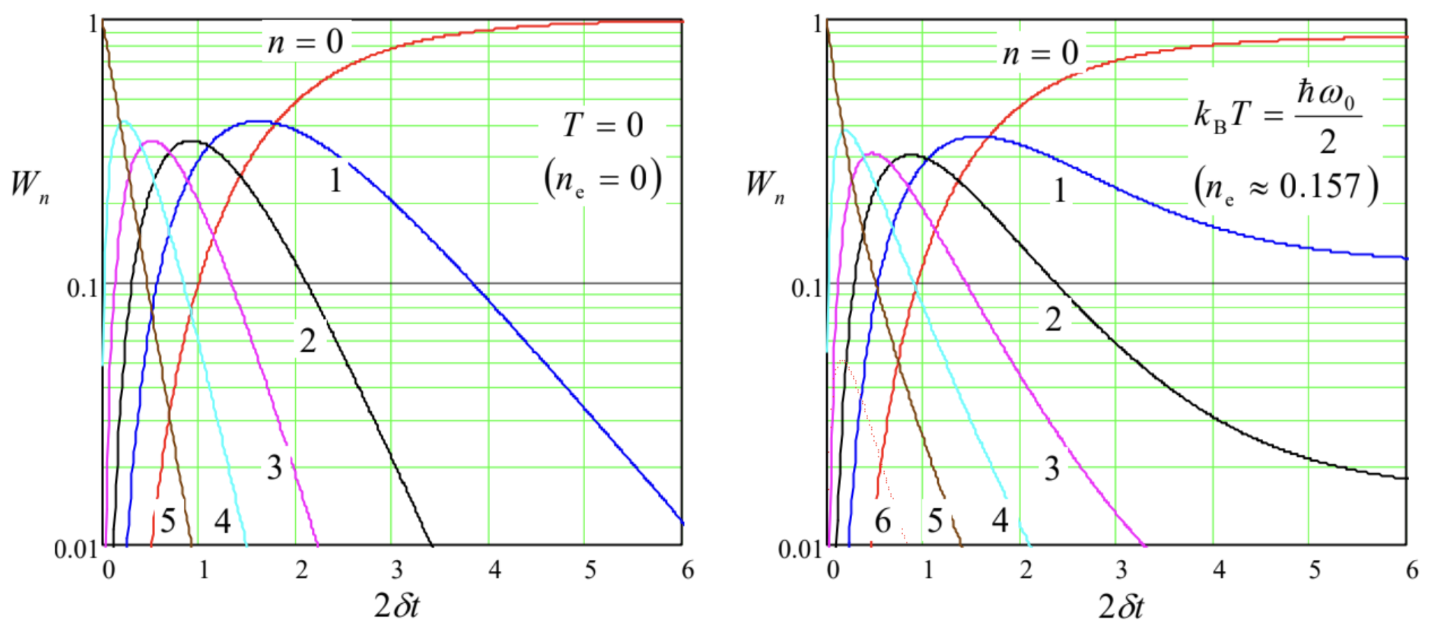
The simple equidistant structure of the oscillator’s spectrum makes it possible to readily solve the system of Eqs. (208), with \(n=0,1,2, \ldots\), for some important cases. In particular, if the initial state of the oscillator is a classical mixture, with no off-diagonal elements, its further relaxation proceeds as such a mixture: \(w_{n n} \cdot(t)=0\) for all \(n^{\prime} \neq n .72\) In particular, it is straightforward to use Eq. (208) to verify that if the initial classical mixture obeys the Gibbs distribution ( 25 ), but with a temperature \(T_{\mathrm{i}}\) different from that of the environment \(\left(T_{\mathrm{e}}\right)\), then the relaxation process is reduced to a simple exponential transient of the effective temperature from \(T_{\mathrm{i}}\) to \(T_{\mathrm{e}}\) : \[W_{n}(t)=\exp \left\{-n \frac{\hbar \omega_{0}}{k_{\mathrm{B}} T_{\mathrm{ef}}(t)}\right\}\left(1-\exp \left\{-\frac{\hbar \omega_{0}}{k_{\mathrm{B}} T_{\mathrm{ef}}(t)}\right\}\right), \quad \text { with } T_{\mathrm{ef}}(t)=T_{\mathrm{i}} e^{-2 \delta t}+T_{\mathrm{e}}\left(1-e^{-2 \delta t}\right),\] with the corresponding evolution of the expectation value of the full energy \(E-\mathrm{cf}\). Eq. (26b): \[\langle E\rangle(t)=\frac{\hbar \omega_{0}}{2}+\hbar \omega_{0}\langle n\rangle(t), \quad\langle n\rangle(t)=\frac{1}{\exp \left\{\hbar \omega_{0} / k_{\mathrm{B}} T_{\mathrm{ef}}(t)\right\}-1} \rightarrow_{t \rightarrow \infty} n_{\mathrm{e}} .\] However, if the initial state of the oscillator is different (say, corresponds to some upper Fock state), the relaxation process, described by Eqs. (208)-(209), is more complex - see, e.g., Fig. 8. At low temperatures (Fig. 8a), it may be interpreted as a gradual "roll" of the probability distribution down the energy staircase, with a gradually decreasing velocity \(d n / d t \propto n\). However, at substantial temperatures, with \(k_{\mathrm{B}} T \sim \hbar \omega_{0}\) (Fig. \(8 \mathrm{~b}\) ), this "roll-down" is saturated when the level occupancies \(W_{n}(t)\) approach their equilibrium values \((25) \cdot{ }^{73}\)

Fig. 7.8. Relaxation of a harmonic oscillator, initially in its \(5^{\text {th }}\) Fock state, at: (a) \(T=0\), and (b) \(T>0\). Note that in the latter case, even the energy levels with \(n>5\) get populated, due to their thermal excitation.

The analysis of this process may be simplified in the case when \(W(n, t) \equiv W_{n}(t)\) is a smooth function of the energy level number \(n\), limited to high levels: \(n \gg>1\). In this limit, we may use the Taylor expansion of this function (written for the points \(\Delta n=\pm 1\) ), truncated to three leading terms: \[W_{n \pm 1}(t) \equiv W(n \pm 1, t) \approx W(n, t) \pm \frac{\partial W(n, t)}{\partial n}+\frac{1}{2} \frac{\partial^{2} W(n, t)}{\partial n^{2}} .\] Plugging this expression into Eqs. (208)-(209), we get for the function \(W(n, t)\) a partial differential equation, which may be recast in the following form: \[\frac{\partial W}{\partial t}=-\frac{\partial}{\partial n}[f(n) W]+\frac{\partial^{2}}{\partial n^{2}}[d(n) W], \quad \text { with } f(n) \equiv 2 \delta\left(n_{\mathrm{e}}-n\right), \quad d(n) \equiv 2 \delta\left(n_{\mathrm{e}}+1 / 2\right) n .\] Since at \(n \gg>1\), the oscillator’s energy \(E\) is close to \(\hbar \omega_{0} n\), this energy diffusion equation (sometimes incorrectly called the Fokker-Planck equation - see below) essentially describes the time evolution of the continuous probability density \(w(E, t)\), which may be defined as \(w(E, t) \equiv W\left(E / \hbar \omega_{0}, t\right) / \hbar \omega_{0} .{ }^{74}\)

This continuous approximation naturally reminds us of the need to discuss dissipative systems with a continuous spectrum. Unfortunately, for such systems the few (relatively :-) simple results that may be obtained from the basic Eq. (181), are essentially classical in nature and are discussed in detail in the SM part of this series. Here, I will give only a simple illustration. Let us consider a 1D particle that interacts weakly with a thermally-equilibrium environment, but otherwise is free to move along the \(x\)-axis. As we know from Chapters 2 and 5 , in this case, the most convenient basis is that of the momentum eigenstates \(p\). In the momentum representation, the density matrix is just the \(c\)-number function \(w\left(p, p^{\prime}\right)\), defined by Eq. (54), which was already discussed in brief in Sec. 2 . On the other hand, the coordinate operator, which participates in the right-hand side of Eq. (181), has the form given by the first of Eqs. (4.269), \[\hat{x}=i \hbar \frac{\partial}{\partial p},\] dual to the coordinate-representation formula (4.268). As we already know, such operators are local see, e.g., Eq. (4.244). Due to this locality, the whole right-hand side of Eq. (181) is local as well, and hence (within the framework of our perturbative treatment) the interaction with the environment affects only the diagonal values \(w(p, p)\) of the density matrix, i.e. the momentum probability density \(w(p)\).

Let us find the equation governing the evolution of this function in time in the Markov approximation, when the time scale of the density matrix evolution is much longer than the correlation time \(\tau_{c}\) of the environment, i.e. the time scale of the functions \(K_{F}(\tau)\) and \(G(\tau)\). In this approximation, we may take the matrix elements out of the first integral of Eq. (181), \[\begin{aligned} &-\frac{1}{\hbar^{2}} \int_{-\infty}^{t} K_{F}\left(t-t^{\prime}\right) d t^{\prime}\left[\hat{x}(t),\left[\hat{x}\left(t^{\prime}\right), \hat{w}\left(t^{\prime}\right)\right]\right] \approx-\frac{1}{\hbar^{2}} \int_{0}^{\infty} K_{F}(\tau) d \tau[\hat{x},[\hat{x}, \hat{w}]] \\ &=-\frac{\pi}{\hbar^{2}} S_{F}(0)[\hat{x},[\hat{x}, \hat{w}]]=-\frac{k_{\mathrm{B}} T}{\hbar^{2}} \eta[\hat{x},[\hat{x}, \hat{w}]], \end{aligned}\] and calculate the last double commutator in the Schrödinger picture. This may be done either using an explicit expression for the matrix elements of the coordinate operator or in a simpler way - using the same trick as at the derivation of the Ehrenfest theorem in Sec. 5.2. Namely, expanding an arbitrary function \(f(p)\) into the Taylor series in \(p\), \[f(p)=\sum_{k=0}^{\infty} \frac{1}{k !} \frac{\partial^{k} f}{\partial p^{k}} p^{k},\] and using Eq. (215), we can prove the following simple commutation relation \[[\hat{x}, f]=\sum_{k=0}^{\infty} \frac{1}{k !} \frac{\partial^{k} f}{\partial p^{k}}\left[\hat{x}, p^{k}\right]=\sum_{k=0}^{\infty} \frac{1}{k !} \frac{\partial^{k} f}{\partial p^{k}}\left(i \hbar k p^{k-1}\right)=i \hbar \sum_{k=1}^{\infty} \frac{1}{(k-1) !} \frac{\partial^{k-1}}{\partial p^{k-1}}\left(\frac{\partial f}{\partial p}\right) p^{k-1}=i \hbar \frac{\partial f}{\partial p} .\] Now applying this result sequentially, first to \(w\) and then to the resulting commutator, we get \[[\hat{x},[\hat{x}, w]]=\left[\hat{x}, i \hbar \frac{\partial w}{\partial p}\right]=i \hbar \frac{\partial}{\partial p}\left(i \hbar \frac{\partial w}{\partial p}\right)=-\hbar^{2} \frac{\partial^{2} w}{\partial p^{2}} .\] It may look like the second integral in Eq. (181) might be simplified similarly. However, it vanishes at \(p^{\prime} \rightarrow p\), and \(t^{\prime} \rightarrow t\), so that to calculate the first non-vanishing contribution from that integral for \(p=p^{\prime}\), we have to take into account the small difference \(\tau \equiv t-t^{\prime} \sim \tau_{\mathrm{c}}\) between the arguments of the coordinate operators under that integral. This may be done using Eq. (169) with the free-particle’s Hamiltonian consisting of the kinetic-energy contribution alone: \[\hat{x}\left(t^{\prime}\right)-\hat{x}(t) \approx-\tau \dot{\hat{x}}=-\tau \frac{1}{i \hbar}\left[\hat{x}, \hat{H}_{s}\right]=-\tau \frac{1}{i \hbar}\left[\hat{x}, \frac{\hat{p}^{2}}{2 m}\right]=-\tau \frac{\hat{p}}{m},\] where the exact argument of the operator on the right-hand side is already unimportant and may be taken for \(t\). As a result, we may use the last of Eqs. (136) to reduce the second term on the right-hand side of Eq. (181) to \[-\frac{i}{2 \hbar} \int_{-\infty}^{t} G\left(t-t^{\prime}\right)\left[\hat{x}(t),\left\{\hat{x}\left(t^{\prime}\right), \hat{w}\left(t^{\prime}\right)\right\}\right] d t^{\prime} \approx \frac{i}{2 \hbar} \int_{0}^{\infty} G(\tau) \tau d \tau\left[\hat{x},\left\{\frac{\hat{p}}{m}, \hat{w}\right\}\right]=\frac{\eta}{2 i \hbar}\left[\hat{x},\left\{\frac{\hat{p}}{m}, \hat{w}\right\}\right] .\] In the momentum representation, the momentum operator and the density matrix \(w\) are just \(c\)-numbers and commute, so that, applying Eq. (218) to the product \(p w\), we get \[\left[\hat{x},\left\{\frac{\hat{p}}{m}, \hat{w}\right\}\right]=\left[\hat{x}, 2 \frac{p}{m} w\right]=2 i \hbar \frac{\partial}{\partial p}\left(\frac{p}{m} w\right),\] and may finally reduce the integro-differential equation Eq. (181) to a partial differential equation: \[\frac{\partial w}{\partial t}=-\frac{\partial}{\partial p}(F w)+\eta k_{\mathrm{B}} T \frac{\partial^{2} w}{\partial p^{2}}, \quad \text { with } F \equiv-\eta \frac{p}{m} .\] This is the 1D form of the famous Fokker-Planck equation describing the classical statistics of motion of a particle (in our particular case, of a free particle) in an environment providing a linear drag characterized by the coefficient \(\eta\); it belongs to the same drift-diffusion type as Eq. (214). The first, drift term on its right-hand side describes the particle’s deceleration due to the drag force \((137), F=-\eta p / m=\) \(-\eta v\), provided by the environment. The second, diffusion term on the right-hand side of Eq. (223) describes the effect of fluctuations: the particle’s momentum’ random walk around its average (driftaffected, and hence time-dependent) value. The walk obeys the law similar to Eq. (85), but with the momentum-space diffusion coefficient \[D_{p}=\eta k_{\mathrm{B}} T\] This is the reciprocal-space version of the fundamental Einstein relation between the dissipation (friction) and fluctuations, in this classical limit represented by their thermal energy scale \(k_{\mathrm{B}} T .^{75}\)

Just for the reader’s reference, let me note that the Fokker-Planck equation (223) may be readily generalized to the 3D motion of a particle under the effect of an additional external force, \({ }^{76}\) and in this more general form is the basis for many important applications; however, due to its classical character, its discussion is also left for the SM part of this series. \({ }^{77}\)

To summarize our discussion of the two alternative approaches to the analysis of quantum systems interacting with a thermally-equilibrium environment, described in the last three sections, let me emphasize again that they give different descriptions of the same phenomena, and are characterized by the same two functions \(G(\tau)\) and \(K_{F}(\tau)\). Namely, in the Heisenberg-Langevin approach, we describe the system by operators that change (fluctuate) in time, even in the thermal equilibrium, while in the density-matrix approach, the system is described by non-fluctuating probability functions, such as \(W_{n}(t)\) or \(w(p, t)\), which are stationary in equilibrium. In the cases when a problem may be solved analytically to the end by both methods (for example, for a harmonic oscillator), they give identical results.

---

\({ }^{54}\) As in Sec. 4, the reader not interested in the derivation of the basic equation (181) of the density matrix evolution may immediately jump to the discussion of this equation and its applications.

\({ }^{55} \mathrm{~A}\) similar analysis of a more general case, when the interaction with the environment has to be represented as a sum of products of the type (90), may be found, for example, in the monograph by \(\mathrm{K}\). Blum, Density Matrix Theory and Applications, \(3^{\text {rd }}\) ed., Springer, \(2012 .\)

\({ }^{56}\) If we used either the Schrödinger or the Heisenberg picture instead, the forthcoming Eq. (175) would pick up a rather annoying multitude of fast-oscillating exponents, of different time arguments, on its right-hand side.

\({ }^{57}\) For the notation simplicity, the fact that here (and in all following formulas) the density operator \(\hat{w}\) of the system \(s\) of our interest is taken in the interaction picture, is just implied.

\({ }^{58}\) Named after Andrey Andreyevich Markov (1856-1922; in older Western literature, "Markoff"), a mathematician famous for his general theory of the so-called Markov processes, whose future development is completely determined by its present state, but not its pre-history.

\({ }^{59}\) Here, rather reluctantly, I will use this standard notation, \(E_{n}\), for the eigenenergies of our system of interest \((s)\), in hope that the reader would not confuse these discrete energy levels with the quasi-continuous energy levels of its environment \((e)\), participating in particular in Eqs. (108) and (111). As a reminder, by this stage of our calculations, the environment levels have disappeared from our formulas, leaving behind their functionals \(K_{F}(\tau)\) and \(G(\tau)\).

\({ }^{60} \mathrm{This}\) is essentially the same rotating-wave approximation (RWA) as was used in Sec. 6.5.

\({ }^{61}\) As was already discussed in Sec. 4 , the lower-limit substitution \(\left(t^{\prime}=-\infty\right)\) in the integrals participating in Eq. (183) gives zero, due to the finite-time "memory" of the system, expressed by the decay of the correlation and response functions at large values of the time delay \(\tau=t-t\) ’.

\({ }^{62}\) The master equations, first introduced to quantum mechanics in 1928 by W. Pauli, are sometimes called the "Pauli master equations", or "kinetic equations", or "rate equations".

\({ }^{63}\) As Eq. (193) shows, the term with \(m=n\) would vanish and thus may be legitimately excluded from the sum.

\({ }^{64}\) As Eq. (193) shows, the result for \(\Gamma_{n \rightarrow n^{\prime}}\) is described by Eq. (195) as well, provided that the indices \(n\) and \(n\) ’ are swapped in all components of its right-hand side, including the swap \(\omega_{n n^{\prime}} \rightarrow \omega_{n^{\prime} n}=-\omega_{n n}\).

\({ }^{65}\) It is straightforward (and highly recommended to the reader) to show that at low temperatures \(\left(k_{\mathrm{B}} T<<\mid E_{n^{\prime}}-\right.\) \(E_{n} \mid\) ), Eq. (196) gives the same result as the Golden Rate formula (6.111), with \(A=x\). (The low-temperature condition ensures that the initial occupancy of the excited level \(n\) is negligible, as was assumed at the derivation of Eq. (6.111).)

\({ }^{66}\) Sometimes Eq. (200) (in any of its numerous alternative forms) is called the Redfield equation, after the 1965 work by A. Redfield. Note, however, that in the mid-1960s several other authors, notably including (in the alphabetical order) H. Haken, W. Lamb, M. Lax, W. Louisell, and M. Scully, also made major contributions to the very fast development of the density-matrix approach to open quantum systems.

\({ }^{67}\) Such corrections are sometimes called Lamb shifts, due to their conceptual similarity to the genuine Lamb shift - the effect first observed experimentally in 1947 by Willis Lamb and Robert Retherford: a minor difference between energy levels of the \(2 s\) and \(2 p\) states of hydrogen, due to the electric-dipole coupling of hydrogen atoms to the free-space electromagnetic environment. (These energies are equal not only in the non-relativistic theory described in Sec. \(3.6\) but also in the relativistic theory (see Secs. 6.3, 9.7), if the electromagnetic environment is ignored.) The explanation of the Lamb shift by H. Bethe, in the same 1947, essentially launched the whole field of quantum electrodynamics - to be briefly discussed in Chapter 9.

\({ }^{68}\) The first form of Eq. (203), as well as the analysis of Sec. 3, implies that low-frequency fluctuations of any other origin, not taken into account in own current analysis (say, an unintentional noise from experimental equipment), may also contribute to dephasing; such "technical fluctuations" are indeed a very serious challenge for the experimental implementation of coherent qubit systems - see Sec. \(8.5\) below.

\({ }^{69}\) As was discussed in Sec. 5.1, the tunneling may be described by using, instead of Eq. (70), the full two-level Hamiltonian (5.3). Let me leave for the reader’s exercise to spell out the equations for the time evolution of the density matrix elements of this system, and of the expectation values of the Pauli operators, for this case.

\({ }^{70}\) This coefficient participates prominently in the classical theory of damped oscillations (see, e.g., CM Sec. 5.1), in particular defining the oscillator’s \(Q\)-factor as \(Q \equiv \omega_{0} / 2 \delta\), and the decay time of the amplitude \(A\) and the energy \(E\) of free oscillations: \(A(t)=A(0) \exp \{-\delta t\}, E(t)=E(0) \exp \{-2 \delta t\}\).

\({ }^{71}\) Sometimes Eq. (207) is called the Lindblad equation, but I believe this terminology is inappropriate. It is true that its structure falls into a general category of equations, suggested by G. Lindblad in 1976 for the density operators in the Markov approximation, whose diagonalized form in the interaction picture is \[\dot{\hat{w}}=\sum_{j} \gamma_{j}\left(2 \hat{L}_{j} \hat{w} \hat{L}_{j}^{\dagger}-\left\{\hat{L}_{j} \hat{L}_{j}^{\dagger}, \hat{w}\right\}\right) .\] However, Eq. (207) was derived much earlier (by L. Landau in 1927 for zero temperature, and by M. Lax in 1960 for an arbitrary temperature), and in contrast to the general Lindblad equation, spells out the participating operators \(\hat{L}_{j}\) and coefficients \(\gamma_{j}\) for a particular physical system - the harmonic oscillator.

\({ }^{72}\) Note, however, that this is not true for many applications, in which a damped oscillator is also under the effect of an external time-dependent field, which may be described by additional, typically off-diagonal terms on the right-hand side of Eqs. (205).

\({ }^{73}\) The reader may like to have a look at the results of nice measurements of such functions \(W_{n}(t)\) in microwave oscillators, performed using their coupling with Josephson-junction circuits: H. Wang et al., Phys. Rev. Lett. 101, 240401 (2008), and with Rydberg atoms: M. Brune et al., Phys. Rev. Lett. 101, 240402 (2008).

\({ }^{74}\) In the classical limit \(n_{\mathrm{e}}>>1\), Eq. (214) is analytically solvable for any initial conditions - see, e.g., the paper by B. Zeldovich et al., Sov. Phys. JETP 28, 308 (1969), which also gives some more intricate solutions of Eqs. (208)-(209). Note, however, that the most important properties of the damped harmonic oscillator (including its relaxation dynamics) may be analyzed simpler by using the Heisenberg-Langevin approach discussed in the previous section.

\({ }^{75}\) Note that Eq. (224), as well as the original Einstein’s relation between the diffusion coefficient \(D\) in the direct space and temperature, may be derived much simpler by other means - for example, from the Nyquist formula (139). These issues are discussed in detail in SM Chapter \(5 .\)

\({ }^{76}\) Moreover, Eq. (223) may be generalized to the motion of a quantum particle in an additional periodic potential \(U(\mathbf{r})\). In this case, due to the band structure of the energy spectrum (which was discussed in Secs. 2.7 and 3.4), the coupling to the environment produces not only a continuous drift-diffusion of the probability density in the space of the quasimomentum \(\hbar \mathbf{q}\) but also quantum transitions between different energy bands at the same \(\hbar \mathbf{q}-\) see, e.g., K. Likharev and A. Zorin, J. Low Temp. Phys. 59, 347 (1985).

\({ }^{77}\) See SM Secs. 5.6-5.7. For a more detailed discussion of quantum effects in dissipative systems with continuous spectra see, e. g., either U. Weiss, Quantum Dissipative Systems, \(2^{\text {nd }}\) ed., World Scientific, 1999, or H.-P. Breuer and F. Petruccione, The Theory of Open Quantum Systems, Oxford U. Press, \(2007 .\)