7.3: Open System Dynamics- Dephasing

So far we have discussed the density operator as something given at a particular time instant. Now let us discuss how is it formed, i.e. its evolution in time, starting from the simplest case when the probabilities \(W_{j}\) participating in Eq. (15) are time-independent-by this or that reason, to be discussed in a moment. In this case, in the Schrödinger picture, we may rewrite Eq. (15) as \[\hat{w}(t)=\sum_{j}\left|w_{j}(t)\right\rangle W_{j}\left\langle w_{j}(t)\right| .\] Taking a time derivative of both sides of this equation, multiplying them by \(i \hbar\), and applying Eq. (4.158) to the basis states \(w_{j}\), with the account of the fact that the Hamiltonian operator is Hermitian, we get \[\begin{aligned} i \hbar \dot{\hat{w}} &=i \hbar \sum_{j}\left(\left|\dot{w}_{j}(t)\right\rangle W_{j}\left\langle w_{j}(t)|+| w_{j}(t)\right\rangle W_{j}\left\langle\dot{w}_{j}(t)\right|\right) \\ &=\sum_{j}\left(\hat{H}\left|w_{j}(t)\right\rangle W_{j}\left\langle w_{j}(t)|-| w_{j}(t)\right\rangle W_{j}\left\langle w_{j}(t)\right| \hat{H}\right) \\ & \equiv \hat{H} \sum_{j}\left|w_{j}(t)\right\rangle W_{j}\left\langle w_{j}(t)\left|-\sum_{j}\right| w_{j}(t)\right\rangle W_{j}\left\langle w_{j}(t)\right| \hat{H} \end{aligned}\] Now using Eq. (64) again (twice), we get the so-called von Neumann equation \(^{22}\) \[i \hbar \dot{\hat{w}}=[\hat{H}, \hat{w}] .\] Note that this equation is similar in structure to Eq. (4.199) describing the time evolution of timeindependent operators in the Heisenberg picture operators: \[i \hbar \dot{\hat{A}}=[\hat{A}, \hat{H}]\] besides the opposite order of the operators in the commutator - equivalent to the change of sign of the right-hand side. This should not be too surprising, because Eq. (66) belongs to the Schrödinger picture of quantum dynamics, while Eq. (67), to its Heisenberg picture.

The most important case when the von Neumann equation is (approximately) valid is when the "own" Hamiltonian \(\hat{H}_{s}\) of the system \(s\) of our interest is time-independent, and its interaction with the environment is so small that its effect on the system’s evolution during the considered time interval is negligible, but it had lasted so long that it gradually put the system into a non-pure state - for example, but not necessarily, into the classical mixture (24). \({ }^{23}\) (This is an example of the second case discussed in Sec. 1, when we need the mixed-ensemble description of the system even if its current interaction with the environment is negligible.) If the interaction with the environment is stronger, and hence is not negligible at the considered time interval, Eq. (66) is generally not valid, \({ }^{24}\) because the probabilities \(W_{j}\) may change in time. However, this equation may still be used for a discussion of one major effect of the environment, namely dephasing (also called "decoherence"), within a simple model.Let us start with the following general model a system interacting with its environment, which will be used throughout this chapter: \[\hat{H}=\hat{H}_{s}+\hat{H}_{e}\{\lambda\}+\hat{H}_{\text {int }}\] where \(\{\lambda\}\) denotes the (huge) set of degrees of freedom of the environment. \({ }^{25}\) Evidently, this model is useful only if we may somehow tame the enormous size of the Hilbert space of these degrees of freedom, and so work out the calculations all way to a practicably simple result. This turns out to be possible mostly if the elementary act of interaction of the system and its environment is in some sense small. Below, I will describe several cases when this is true; the classical example is the Brownian particle interacting with the molecules of the surrounding gas or fluid. \({ }^{26}\) (In this example, a single hit by a molecule changes the particle’s momentum by a minor fraction.) On the other hand, the model (68) is not very productive for a particle interacting with the environment consisting of similar particles, when a single collision may change its momentum dramatically. In such cases, the methods discussed in the next chapter are more relevant.

Now let us analyze a very simple model of an open two-level quantum system, with its intrinsic Hamiltonian having the form \[\hat{H}_{s}=c_{z} \hat{\sigma}_{z},\] similar to the Pauli Hamiltonian (4.163), \({ }^{27}\) and a factorable, bilinear interaction - cf. Eq. (6.145) and its discussion: \[\hat{H}_{\text {int }}=\hat{f}\{\lambda\} \hat{\sigma}_{z},\] where \(\hat{f}\) is a Hermitian operator depending only on the set \(\{\lambda\}\) of environmental degrees of freedom ("coordinates"), defined in their Hilbert space - different from that of the two-level system. As a result, the operators \(\hat{f}\{\lambda\}\) and \(\hat{H}_{e}\{\lambda\}\) commute with \(\hat{\sigma}_{z}\) - and with any other intrinsic operator of the two-level system. Of course, any realistic \(\hat{H}_{e}\{\lambda\}\) is extremely complex, so that how much we will be able to achieve without specifying it, may be a pleasant surprise for the reader.Before we proceed to the analysis, let us recognize two examples of two-level systems that may be described by this model. The first example is a spin- \(1 / 2\) in an external magnetic field of a fixed direction (taken for the axis \(z\) ), which includes both an average component \(\overline{\mathcal{B}}\) and a random (fluctuating) component \(\widetilde{\mathcal{B}_{z}}(t)\) induced by the environment. As it follows from Eq. (4.163b), it may be described by the Hamiltonian (68)-(70) with \[c_{z}=-\frac{\hbar \gamma}{2} \overline{\mathscr{B}}_{z}, \quad \text { and } \quad \hat{f}=-\frac{\hbar \gamma}{2} \overbrace{\widetilde{B}_{z}}(t) .\] Another example is a particle in a symmetric double-well potential \(U_{s}\) (Fig. 4), with a barrier between them sufficiently high to be practically impenetrable, and an additional force \(F(t)\), exerted by the environment, so that the total potential energy is \(U(x, t)=U_{s}(x)-F(t) x\). If the force, including its static part \(\bar{F}\) and fluctuations \(\widetilde{F}(t)\), is sufficiently weak, we can neglect its effects on the shape of potential wells and hence on the localized wavefunctions \(\psi_{\mathrm{L}, \mathrm{R}}\), so that the force effect is reduced to the variation of the difference \(E_{\mathrm{L}}-E_{\mathrm{R}}=F(t) \Delta x\) between the eigenenergies. As a result, the system may be described by Eqs. (68)-(70) with \[c_{z}=-\bar{F} \Delta x / 2 ; \quad \hat{f}=-\hat{\widetilde{F}}(t) \Delta x / 2 .\]

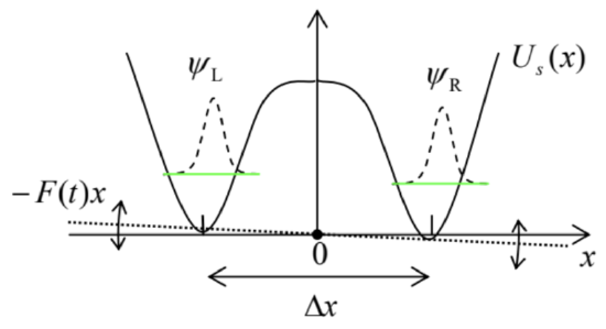Fig. 7.4. Dephasing in a double-well system.

Let us start our general analysis of the model described by Eqs. (68)-(70) by writing the equation of motion for the Heisenberg operator \(\hat{\sigma}_{z}(t)\) : \[i \hbar \dot{\hat{\sigma}}_{z}=\left[\hat{\sigma}_{z}, \hat{H}\right]=\left(c_{z}+\hat{f}\right)\left[\hat{\sigma}_{z}, \hat{\sigma}_{z}\right]=0,\] showing that in our simple model (68)-(70), the operator \(\hat{\sigma}_{z}\) does not evolve in time. What does this mean for the observables? For an arbitrary density matrix of any two-level system, \[w=\left(\begin{array}{ll} w_{11} & w_{12} \\ w_{21} & w_{22} \end{array}\right),\] we can readily calculate the trace of operator \(\hat{\sigma}_{z} \hat{w}\). Indeed, since the operator traces are basisindependent, we can do this in any basis, in particular in the usual \(z\)-basis: \[\operatorname{Tr}\left(\hat{\sigma}_{z} \hat{w}\right)=\operatorname{Tr}\left(\sigma_{z} \mathrm{w}\right)=\operatorname{Tr}\left[\left(\begin{array}{cc} 1 & 0 \\ 0 & -1 \end{array}\right)\left(\begin{array}{cc} w_{11} & w_{12} \\ w_{21} & w_{22} \end{array}\right)\right]=w_{11}-w_{22}=W_{1}-W_{2} .\] Since, according to Eq. (5), \(\hat{\sigma}_{z}\) may be considered the operator for the difference of the number of particles in the basis states 1 and 2 , in the case \((73)\) the difference \(W_{1}-W_{2}\) does not depend on time, and since the sum of these probabilities is also fixed, \(W_{1}+W_{2}=1\), both of them are constant. The physics of this simple result is especially clear for the model shown in Fig. 4: since the potential barrier separating the potential wells is so high that tunneling through it is negligible, the interaction with the environment cannot move the system from one well into another one.

It may look like nothing interesting may happen in such a simple situation, but in a minute we will see that this is not true. Due to the time independence of \(W_{1}\) and \(W_{2}\), we may use the von Neumann equation (66) to describe the density matrix evolution. In the usual \(z\)-basis: \[\begin{aligned} i \hbar \dot{\mathrm{w}} & \equiv i \hbar\left(\begin{array}{ll} \dot{w}_{11} & \dot{w}_{12} \\ \dot{w}_{21} & \dot{w}_{22} \end{array}\right)=[\mathrm{H}, \mathrm{w}] \equiv\left(c_{z}+\hat{f}\right)\left[\sigma_{z}, \mathrm{w}\right] \\ & \equiv\left(c_{z}+\hat{f}\right)\left[\left(\begin{array}{cc} 1 & 0 \\ 0 & -1 \end{array}\right),\left(\begin{array}{ll} w_{11} & w_{12} \\ w_{21} & w_{22} \end{array}\right)\right]=\left(c_{z}+\hat{f}\right)\left(\begin{array}{cc} 0 & 2 w_{12} \\ -2 w_{21} & 0 \end{array}\right) . \end{aligned}\] This result means that while the diagonal elements, i.e., the probabilities of the states, do not evolve in time (as we already know), the off-diagonal elements do change; for example, \[i \hbar \dot{w}_{12}=2\left(c_{z}+\hat{f}\right) w_{12},\] with a similar but complex-conjugate equation for \(w_{21}\). The solution of this linear differential equation (77) is straightforward, and yields \[w_{12}(t)=w_{12}(0) \exp \left\{-i \frac{2 c_{z}}{\hbar} t\right\} \exp \left\{-i \frac{2}{\hbar} \int_{0}^{t} \hat{f}\left(t^{\prime}\right) d t^{\prime}\right\} .\] The first exponent is a deterministic \(c\)-number factor, while in the second one \(\hat{f}(t) \equiv \hat{f}\{\lambda(t)\}\) is still an operator in the Hilbert space of the environment, but from the point of view of the two-level system of our interest, it is a random function of time. The time-average part of this function may be included in \(c_{z}\), so in what follows, we will assume that it equals zero.

Let us start from the limit when the environment behaves classically. \({ }^{28}\) In this case, the operator in Eq. (78) may be considered as a classical random function of time \(f(t)\), provided that we average its effects over a statistical ensemble of many functions \(f(t)\) describing many (macroscopically similar) experiments. For a small time interval \(t=d t \rightarrow 0\), we can use the Taylor expansion of the exponent, truncating it after the quadratic term: \[\begin{aligned} \left\langle\exp \left\{-i \frac{2}{\hbar} \int_{0}^{d t} f\left(t^{\prime}\right) d t^{\prime}\right\}\right.& \approx 1+\left\langle-i \frac{2}{\hbar} \int_{0}^{d t} f\left(t^{\prime}\right) d t^{\prime}\right\rangle+\left\langle\frac{1}{2}\left(-i \frac{2}{\hbar} \int_{0}^{d t} f\left(t^{\prime}\right) d t^{\prime}\right)\left(-i \frac{2}{\hbar} \int_{0}^{d t} f\left(t^{\prime \prime}\right) d t^{\prime \prime}\right)\right\rangle \\ & \equiv 1-i \frac{2}{\hbar} \int_{0}^{d t}\left\langle f\left(t^{\prime}\right)\right\rangle d t^{\prime}-\frac{2}{\hbar^{2}} \int_{0}^{d t} d t^{\prime} \int_{0}^{d t} d t^{\prime \prime}\left\langle f\left(t^{\prime}\right) f\left(t^{\prime \prime}\right)\right\rangle \equiv 1-\frac{2}{\hbar^{2}} \int_{0}^{d t} d t^{d t} \int_{0}^{d t} d t^{\prime \prime} K_{f}\left(t^{\prime}-t^{\prime \prime}\right) . \end{aligned}\] Here we have used the facts that the statistical average of \(f(t)\) is equal to zero, while the second average, called the correlation function, in a statistically- (i.e. macroscopically-) stationary state of any environment may only depend on the time difference \(\tau \equiv t^{\prime}-t^{\prime \prime}\) : \[\left\langle f\left(t^{\prime}\right) f\left(t^{\prime \prime}\right)\right\rangle=K_{f}\left(t^{\prime}-t^{\prime \prime}\right) \equiv K_{f}(\tau) .\] If this difference is much larger than some time scale \(\tau_{\mathrm{c}}\), called the correlation time of the environment, the values \(f\left(t^{\prime}\right)\) and \(f\left(t^{\prime \prime}\right)\) are completely independent (uncorrelated), as illustrated in Fig. \(5 \mathrm{a}\), so that at \(\tau\) \(\rightarrow \infty\), the correlation function has to tend to zero. On the other hand, at \(\tau=0\), i.e. \(t\) ’ \(=t\) ", the correlation function is just the variance of \(f\) :

\[K_{f}(0)=\left\langle f^{2}\right\rangle,\] and has to be positive. As a result, the function looks (semi-quantitatively) as shown in Fig. \(5 \mathrm{~b}\).

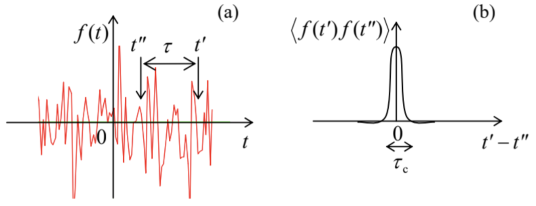Fig. 7.5. (a) A typical random process and (b) its correlation function - schematically.

Hence, if we are only interested in time differences \(\tau\) much longer than \(\tau_{\mathrm{c}}\), which is typically very short, we may approximate \(K_{f}(\tau)\) well with a delta function of the time difference. Let us take it in the following form, convenient for later discussion: \[K_{f}(\tau) \approx \hbar^{2} D_{\varphi} \delta(\tau),\] where \(D_{\varphi}\) is a positive constant called the phase diffusion coefficient. The origin of this term stems from the very similar effect of classical diffusion of Brownian particles in a highly viscous medium. Indeed, the particle’s velocity in such a medium is approximately proportional to the external force. Hence, if the random hits of a particle by the medium’s molecules may be described by a force that obeys a law similar to Eq. (82), the velocity (along any Cartesian coordinate) is also delta-correlated: \[\langle v(t)\rangle=0, \quad\left\langle v\left(t^{\prime}\right) v\left(t^{\prime \prime}\right)\right\rangle=2 D \delta\left(t^{\prime}-t^{\prime \prime}\right) .\] Now we can integrate the kinematic relation \(\dot{x}=v\), to calculate particle’s displacement from its initial position during a time interval \([0, t]\) and its variance: \[\begin{gathered} x(t)-x(0)=\int_{0}^{t} v\left(t^{\prime}\right) d t^{\prime}, \\ \left\langle(x(t)-x(0))^{2}\right\rangle=\left\langle\int_{0}^{t} v\left(t^{\prime}\right) d t^{t} \int_{0}^{t} v\left(t^{\prime \prime}\right) d t^{\prime \prime}\right\rangle=\int_{0}^{t} d t^{t} \int_{0}^{t} d t^{\prime \prime}\left\langle v\left(t^{\prime}\right) v\left(t^{\prime \prime}\right)\right\rangle=\int_{0}^{t} d t^{\prime} \int_{0}^{t} d t^{\prime \prime} 2 D \delta\left(t^{\prime}-t^{\prime \prime}\right)=2 D t . \end{gathered}\] This is the famous law of diffusion, showing that the r.m.s. deviation of the particle from the initial point grows with time as \((2 D t)^{1 / 2}\), where the constant \(D\) is called the diffusion coefficient.

Returning to the diffusion of the quantum-mechanical phase, with Eq. (82) the last double integral in Eq. (79) yields \(\hbar^{2} D_{\varphi} d t\), so that the statistical average of Eq. (78) is \[\left\langle w_{12}(d t)\right\rangle=w_{12}(0) \exp \left\{-i \frac{2 c_{z}}{\hbar} d t\right\}\left(1-2 D_{\varphi} d t\right) .\] Applying this formula to sequential time intervals, \[\left\langle w_{12}(2 d t)\right\rangle=\left\langle w_{12}(d t)\right\rangle \exp \left\{-i \frac{2 c_{z}}{\hbar} d t\right\}\left(1-2 D_{\varphi} d t\right)=w_{12}(0) \exp \left\{-i \frac{2 c_{z}}{\hbar} 2 d t\right\}\left(1-2 D_{\varphi} d t\right)^{2},\] etc., for a finite time \(t=N d t\), in the limit \(N \rightarrow \infty\) and \(d t \rightarrow 0\) (at fixed \(t\) ) we get \[\left\langle w_{12}(t)\right\rangle=w_{12}(0) \exp \left\{-i \frac{2 c_{z}}{\hbar} t\right\} \times \lim _{N \rightarrow \infty}\left(1-2 D_{\varphi} t \frac{1}{N}\right)^{N} .\] By the definition of the natural logarithm base \(e,{ }^{29}\) this limit is just \(\exp \left\{-2 D_{\varphi} t\right\}\), so that, finally: \[\left\langle w_{12}(t)\right\rangle=w_{12}(0) \exp \left\{-i \frac{2 a}{\hbar} t\right\} \exp \left\{-2 D_{\varphi} t\right\} \equiv w_{12}(0) \exp \left\{-i \frac{2 a}{\hbar} t\right\} \exp \left\{-\frac{t}{T_{2}}\right\} .\] So, due to coupling to the environment, the off-diagonal elements of the density matrix decay with some dephasing time \(T_{2}=1 / 2 D_{\varphi}\), providing a natural evolution from the density matrix (22) of a pure state to the diagonal matrix (23), with the same probabilities \(W_{1,2}\), describing a fully dephased (incoherent) classical mixture. \({ }^{30}\)

This simple model offers a very clear look at the nature of the decoherence: the random "force" \(f(t)\), exerted by the environment, "shakes" the energy difference between two eigenstates of the system and hence the instantaneous velocity \(2\left(c_{z}+f\right) / \hbar\) of their mutual phase shift \(\varphi(t)-\) cf. Eq. (22). Due to the randomness of the force, \(\varphi(t)\) performs a random walk around the trigonometric circle, so that the average of its trigonometric functions \(\exp \{\pm i \varphi\}\) over time gradually tends to zero, killing the offdiagonal elements of the density matrix. Our analysis, however, has left open two important issues:

(i) Is this approach valid for a quantum description of a typical environment?

(ii) If yes, what is physically the \(D_{\varphi}\) that was formally defined by Eq. (82)?

---

\({ }^{22}\) In some texts, it is called the "Liouville equation", due to its philosophical proximity to the classical Liouville theorem for the classical distribution function \(w_{\mathrm{cl}}(X, P)\) - see, e.g., SM Sec. \(6.1\) and in particular Eq. (6.5).

\({ }^{23}\) In the last case, the statistical operator is diagonal in the stationary state basis and hence commutes with the Hamiltonian. Hence the right-hand side of Eq. (66) vanishes, and it shows that in this basis, the density matrix is completely time-independent.

\({ }^{24}\) Very unfortunately, this fact is not explained in some textbooks, which quote the von Neumann equation without proper qualifications.

\({ }^{25}\) Note that by writing Eq. (68), we are treating the whole system, including the environment, as a Hamiltonian one. This can always be done if the accounted part of the environment is large enough so that the processes in the system \(s\) of our interest do not depend on the type of boundary between this part and the "external" (even larger) environment; in particular, we may assume the total system to be closed, i.e. Hamiltonian.

\({ }^{26}\) The theory of the Brownian motion, the effect first observed experimentally by biologist Robert Brown in the \(1820 \mathrm{~s}\), was pioneered by Albert Einstein in 1905 and developed in detail by Marian Smoluchowski in 1906-1907 and Adriaan Fokker in 1913. Due to this historic background, in some older texts, the approach described in the balance of this chapter is called the "quantum theory of the Brownian motion". Let me, however, emphasize that due to the later progress of experimental techniques, quantum-mechanical behaviors, including the environmental effects in them, have been observed in a rapidly growing number of various quasi-macroscopic systems, for which this approach is quite applicable. In particular, this is true for most systems being explored as possible qubits of prospective quantum computing and encryption systems - see Sec. \(8.5\) below.

\({ }^{27}\) As we know from Secs. \(4.6\) and 5.1, such Hamiltonian is sufficient to lift the energy level degeneracy.

\({ }^{28}\) This assumption is not in contradiction with the need for the quantum treatment of the two-level system \(s\), because a typical environment is large, and hence has a very dense energy spectrum, with the distances adjacent levels that may be readily bridged by thermal excitations of small energies, often making it essentially classical.

\({ }^{29}\) See, e.g., MA Eq. (1.2a) with \(n=-N / 2 D_{\varnothing} t\).

\({ }^{30}\) Note that this result is valid only if the approximation (82) may be applied at time interval \(d t\) which, in turn, should be much smaller than the \(T_{2}\) in Eq. (88), i.e. if the dephasing time is much longer than the environment’s correlation time \(\tau_{\mathrm{c}}\). This requirement may be always satisfied by making the coupling to the environment sufficiently weak. In addition, in typical environments, \(\tau_{\mathrm{c}}\) is very short. For example, in the original Brownian motion experiments with a-few- \(\mu \mathrm{m}\) pollen grains in water, it is of the order of the average interval between sequential molecular impacts, of the order of \(10^{-21} \mathrm{~s}\).