
6.2: Potential step


- Last updated
- Nov 29, 2021
- Save as PDF

( \newcommand{\kernel}{\mathrm{null}\,}\)
Consider a potential step
V(x)={V0x<aV1x>a
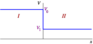
Figure 6.2.1: The step potential discussed in the text
Let me define
k0=√2mℏ2(E−V0),k1=√2mℏ2(E−V1).
I assume a beam of particles comes in from the left,
ϕ(x)=A0eik0xfor x<0.
At the potential step the particles either get reflected back to region I, or are transmitted to region II. There can thus only be a wave moving to the right in region II, but in region I we have both the incoming and a reflected wave,
ϕI(x)=A0eik0x+B0e−ik0x,ϕII(x)=A1eik1x.
We define a transmission (T) and reflection (R) coefficient as the ratio of currents between reflected or transmitted wave and the incoming wave, where we have canceled a common factor
R=|B0|2|A0|2T=k1|A1|2k0|A0|2.
Even though we have given up normalisability, we still have the two continuity conditions. At x=0 these imply, using continuity of ϕ and ddxϕ,
A0+B0=A1,ik0(A0−B0)=ik1A1.
We thus find
A1=2k0k0+k1A0B0=k0−k1k0+k1A0,
and the reflection and transmission coefficients can thus be expressed as
R=(k0−k1k0+k1)2,T=4k1k0(k0+k1)2.
Notice that R+T=1!
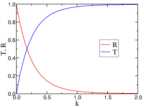
Figure 6.2.2: The transmission and reflection coefficients for a square barrier.
In Figure 6.2.2 we have plotted the behaviour of the transmission and reflection of a beam of Hydrogen atoms impinging on a barrier of height 2 meV.