
5.4: Curvature in Two Spacelike Dimensions
- Page ID
- 11464

\( \newcommand{\vecs}[1]{\overset { \scriptstyle \rightharpoonup} {\mathbf{#1}} } \)
\( \newcommand{\vecd}[1]{\overset{-\!-\!\rightharpoonup}{\vphantom{a}\smash {#1}}} \)
\( \newcommand{\dsum}{\displaystyle\sum\limits} \)
\( \newcommand{\dint}{\displaystyle\int\limits} \)
\( \newcommand{\dlim}{\displaystyle\lim\limits} \)
\( \newcommand{\id}{\mathrm{id}}\) \( \newcommand{\Span}{\mathrm{span}}\)
( \newcommand{\kernel}{\mathrm{null}\,}\) \( \newcommand{\range}{\mathrm{range}\,}\)
\( \newcommand{\RealPart}{\mathrm{Re}}\) \( \newcommand{\ImaginaryPart}{\mathrm{Im}}\)
\( \newcommand{\Argument}{\mathrm{Arg}}\) \( \newcommand{\norm}[1]{\| #1 \|}\)
\( \newcommand{\inner}[2]{\langle #1, #2 \rangle}\)
\( \newcommand{\Span}{\mathrm{span}}\)
\( \newcommand{\id}{\mathrm{id}}\)
\( \newcommand{\Span}{\mathrm{span}}\)
\( \newcommand{\kernel}{\mathrm{null}\,}\)
\( \newcommand{\range}{\mathrm{range}\,}\)
\( \newcommand{\RealPart}{\mathrm{Re}}\)
\( \newcommand{\ImaginaryPart}{\mathrm{Im}}\)
\( \newcommand{\Argument}{\mathrm{Arg}}\)
\( \newcommand{\norm}[1]{\| #1 \|}\)
\( \newcommand{\inner}[2]{\langle #1, #2 \rangle}\)
\( \newcommand{\Span}{\mathrm{span}}\) \( \newcommand{\AA}{\unicode[.8,0]{x212B}}\)
\( \newcommand{\vectorA}[1]{\vec{#1}} % arrow\)
\( \newcommand{\vectorAt}[1]{\vec{\text{#1}}} % arrow\)
\( \newcommand{\vectorB}[1]{\overset { \scriptstyle \rightharpoonup} {\mathbf{#1}} } \)
\( \newcommand{\vectorC}[1]{\textbf{#1}} \)
\( \newcommand{\vectorD}[1]{\overrightarrow{#1}} \)
\( \newcommand{\vectorDt}[1]{\overrightarrow{\text{#1}}} \)
\( \newcommand{\vectE}[1]{\overset{-\!-\!\rightharpoonup}{\vphantom{a}\smash{\mathbf {#1}}}} \)
\( \newcommand{\vecs}[1]{\overset { \scriptstyle \rightharpoonup} {\mathbf{#1}} } \)
\(\newcommand{\longvect}{\overrightarrow}\)
\( \newcommand{\vecd}[1]{\overset{-\!-\!\rightharpoonup}{\vphantom{a}\smash {#1}}} \)
\(\newcommand{\avec}{\mathbf a}\) \(\newcommand{\bvec}{\mathbf b}\) \(\newcommand{\cvec}{\mathbf c}\) \(\newcommand{\dvec}{\mathbf d}\) \(\newcommand{\dtil}{\widetilde{\mathbf d}}\) \(\newcommand{\evec}{\mathbf e}\) \(\newcommand{\fvec}{\mathbf f}\) \(\newcommand{\nvec}{\mathbf n}\) \(\newcommand{\pvec}{\mathbf p}\) \(\newcommand{\qvec}{\mathbf q}\) \(\newcommand{\svec}{\mathbf s}\) \(\newcommand{\tvec}{\mathbf t}\) \(\newcommand{\uvec}{\mathbf u}\) \(\newcommand{\vvec}{\mathbf v}\) \(\newcommand{\wvec}{\mathbf w}\) \(\newcommand{\xvec}{\mathbf x}\) \(\newcommand{\yvec}{\mathbf y}\) \(\newcommand{\zvec}{\mathbf z}\) \(\newcommand{\rvec}{\mathbf r}\) \(\newcommand{\mvec}{\mathbf m}\) \(\newcommand{\zerovec}{\mathbf 0}\) \(\newcommand{\onevec}{\mathbf 1}\) \(\newcommand{\real}{\mathbb R}\) \(\newcommand{\twovec}[2]{\left[\begin{array}{r}#1 \\ #2 \end{array}\right]}\) \(\newcommand{\ctwovec}[2]{\left[\begin{array}{c}#1 \\ #2 \end{array}\right]}\) \(\newcommand{\threevec}[3]{\left[\begin{array}{r}#1 \\ #2 \\ #3 \end{array}\right]}\) \(\newcommand{\cthreevec}[3]{\left[\begin{array}{c}#1 \\ #2 \\ #3 \end{array}\right]}\) \(\newcommand{\fourvec}[4]{\left[\begin{array}{r}#1 \\ #2 \\ #3 \\ #4 \end{array}\right]}\) \(\newcommand{\cfourvec}[4]{\left[\begin{array}{c}#1 \\ #2 \\ #3 \\ #4 \end{array}\right]}\) \(\newcommand{\fivevec}[5]{\left[\begin{array}{r}#1 \\ #2 \\ #3 \\ #4 \\ #5 \\ \end{array}\right]}\) \(\newcommand{\cfivevec}[5]{\left[\begin{array}{c}#1 \\ #2 \\ #3 \\ #4 \\ #5 \\ \end{array}\right]}\) \(\newcommand{\mattwo}[4]{\left[\begin{array}{rr}#1 \amp #2 \\ #3 \amp #4 \\ \end{array}\right]}\) \(\newcommand{\laspan}[1]{\text{Span}\{#1\}}\) \(\newcommand{\bcal}{\cal B}\) \(\newcommand{\ccal}{\cal C}\) \(\newcommand{\scal}{\cal S}\) \(\newcommand{\wcal}{\cal W}\) \(\newcommand{\ecal}{\cal E}\) \(\newcommand{\coords}[2]{\left\{#1\right\}_{#2}}\) \(\newcommand{\gray}[1]{\color{gray}{#1}}\) \(\newcommand{\lgray}[1]{\color{lightgray}{#1}}\) \(\newcommand{\rank}{\operatorname{rank}}\) \(\newcommand{\row}{\text{Row}}\) \(\newcommand{\col}{\text{Col}}\) \(\renewcommand{\row}{\text{Row}}\) \(\newcommand{\nul}{\text{Nul}}\) \(\newcommand{\var}{\text{Var}}\) \(\newcommand{\corr}{\text{corr}}\) \(\newcommand{\len}[1]{\left|#1\right|}\) \(\newcommand{\bbar}{\overline{\bvec}}\) \(\newcommand{\bhat}{\widehat{\bvec}}\) \(\newcommand{\bperp}{\bvec^\perp}\) \(\newcommand{\xhat}{\widehat{\xvec}}\) \(\newcommand{\vhat}{\widehat{\vvec}}\) \(\newcommand{\uhat}{\widehat{\uvec}}\) \(\newcommand{\what}{\widehat{\wvec}}\) \(\newcommand{\Sighat}{\widehat{\Sigma}}\) \(\newcommand{\lt}{<}\) \(\newcommand{\gt}{>}\) \(\newcommand{\amp}{&}\) \(\definecolor{fillinmathshade}{gray}{0.9}\)Since the curvature tensors in 3+1 dimensions are complicated, let’s start by considering lower dimensions. In one dimension, Figure 5.3.1, there is no such thing as intrinsic curvature. This is because curvature describes the failure of parallelism to behave as in E5, but there is no notion of parallelism in one dimension.
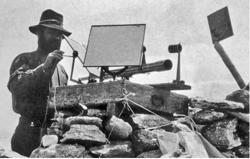
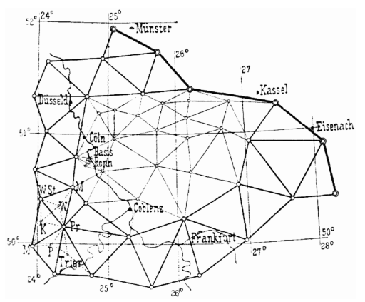
The lowest interesting dimension is therefore two, and this case was studied by Carl Friedrich Gauss in the early nineteenth century. Gauss ran a geodesic survey of the state of Hanover, inventing an optical surveying instrument called a heliotrope that in effect was used to cover the Earth’s surface with a triangular mesh of light rays. If one of the mesh points lies, for example, at the peak of a mountain, then the sum \(\Sigma \theta\) of the angles of the vertices meeting at that point will be less than 2\(\pi\), in contradiction to Euclid. Although the light rays do travel through the air above the dirt, we can think of them as approximations to geodesics painted directly on the dirt, which would be intrinsic rather than extrinsic. The angular defect around a vertex now vanishes, because the space is locally Euclidean, but we now pick up a different kind of angular defect, which is that the interior angles of a triangle no longer add up to the Euclidean value of \(\pi\).
Example 1: A polygonal survey of a soccer ball
Figure 5.3.3 applies similar ideas to a soccer ball, the only difference being the use of pentagons and hexagons rather than triangles.
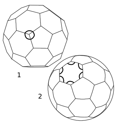
In Figure 5.3.4 (1), the survey is extrinsic, because the lines pass below the surface of the sphere. The curvature is detectable because the angles at each vertex add up to 120 + 120 + 110 = 350 degrees, giving an angular defect of 10 degrees.
In Figure 5.3.4 (2), the lines have been projected to form arcs of great circles on the surface of the sphere. Because the space is locally Euclidean, the sum of the angles at a vertex has its Euclidean value of 360 degrees. The curvature can be detected, however, because the sum of the internal angles of a polygon is greater than the Euclidean value. For example, each spherical hexagon gives a sum of 6 × 124.31 degrees, rather than the Euclidean 6 × 120. The angular defect of 6 × 4.31 degrees is an intrinsic measure of curvature.
Example 2: Angular defect on the earth’s surface
Divide the Earth’s northern hemisphere into four octants, with their boundaries running through the north pole. These octants have sides that are geodesics, so they are equilateral triangles. Assuming Euclidean geometry, the interior angles of an equilateral triangle are each equal to 60 degrees, and, as with any triangle, they add up to 180 degrees. The octant-triangle in Figure 5.3.5 has angles that are each 90 degrees, and the sum is 270. This shows that the Earth’s surface has intrinsic curvature.
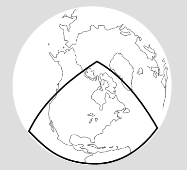
This example suggests another way of measuring intrinsic curvature, in terms of the ratio \(\frac{C}{r}\) of the circumference of a circle to its radius. In Euclidean geometry, this ratio equals 2\(\pi\). Let \(\rho\) be the radius of the Earth, and consider the equator to be a circle centered on the north pole, so that its radius is the length of one of the sides of the triangle in Figure 5.3.5, \(r = (\frac{\pi}{2}) \rho\). (Don’t confuse r, which is intrinsic, with \(\rho\), the radius of the sphere, which is extrinsic and not equal to r.) Then the ratio \(\frac{C}{r}\) is equal to 4, which is smaller than the Euclidean value of 2\(\pi\).
Let
\[\epsilon = \sum \theta − \pi\]
be the angular defect of a triangle, and for concreteness let the triangle be in a space with an elliptic geometry, so that it has constant curvature and can be modeled as a sphere of radius \(\rho\), with antipodal points identified.
Exercise \(\PageIndex{1}\)
In elliptic geometry, what is the minimum possible value of the quantity \(\frac{C}{r}\) discussed in example 2? How does this differ from the case of spherical geometry?
We want a measure of curvature that is local, but if our space is locally flat, we must have \(\epsilon → 0\) as the size of the triangles approaches zero. This is why Euclidean geometry is a good approximation for small-scale maps of the earth. The discrete nature of the triangular mesh is just an artifact of the definition, so we want a measure of curvature that, unlike \(\epsilon\), approaches some finite limit as the scale of the triangles approaches zero. Should we expect this scaling to go as \(\epsilon \propto \rho\)? \(\rho^{2}\)? Let’s determine the scaling. First we prove a classic lemma by Gauss, concerning a slightly different version of the angular defect, for a single triangle.
Theorem
In elliptic geometry, the angular defect \(\epsilon = \alpha + \beta + \gamma − \pi\) of a triangle is proportional to its area A.
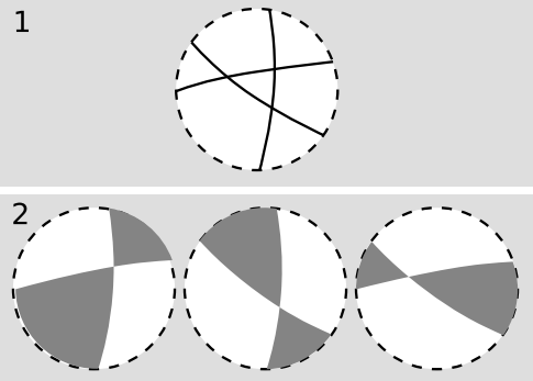
proof
By axiom E2, extend each side of the triangle to form a line, Figure 5.3.6 (1). Each pair of lines crosses at only one point (E1) and divides the plane into two lunes with their four vertices touching at this point, Figure 5.3.6 (2). Of the six lunes, we focus on the three shaded ones, which overlap the triangle. In each of these, the two interior angles at the vertex are the same (Euclid I.15). The area of a lune is proportional to its interior angle, as follows from dissection into narrower lunes; since a lune with an interior angle of \(\pi\) covers the entire area P of the plane, the constant of proportionality is \(\frac{P}{\pi}\). The sum of the areas of the three lunes is \((\frac{P}{\pi})(\alpha + \beta + \gamma)\), but these three areas also cover the entire plane, overlapping three times on the given triangle, and therefore their sum also equals \(P + 2A\). Equating the two expressions leads to the desired result.
This calculation was purely intrinsic, because it made no use of any model or coordinates. We can therefore construct a measure of curvature that we can be assured is intrinsic, \(K = \frac{\epsilon}{A}\). This is called the Gaussian curvature, and in elliptic geometry it is constant rather than varying from point to point. In the model on a sphere of radius \(\rho\), we have
\[K = \frac{1}{\rho^{2}}.\]
Exercise \(\PageIndex{2}\)
Self-check: Verify the equation \(K = \frac{1}{\rho^{2}}\) by considering a triangle covering one octant of the sphere, as in example 2.
Gaussian Normal Coordinates
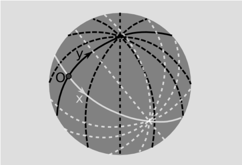
It is useful to introduce normal or Gaussian normal coordinates, defined as follows. Through point O, construct perpendicular geodesics, and define affine coordinates x and y along these. For any point P off the axis, define coordinates by constructing the lines through P that cross the axes perpendicularly. For P in a sufficiently small neighborhood of O, these lines exist and are uniquely determined. Gaussian polar coordinates can be defined in a similar way.
Here are two useful interpretations of K.
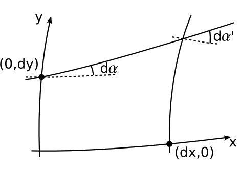
- The Gaussian curvature measures the failure of parallelism in the following sense. Let line \(\ell\) be constructed so that it crosses the normal y axis at (0, dy) at an angle that differs from perpendicular by the infinitesimal amount d\(\alpha\) (Figure 5.3.8). Construct the line x' = dx, and let d\(\alpha'\) be the angle its perpendicular forms with \(\ell\). Then1 the Gaussian curvature at O is $$K = \frac{d^{2} \alpha}{dx dy},$$where \(d^{2} \alpha = d \alpha' - d \alpha\).
Proof
Since any two lines cross in elliptic geometry, \(\ell\) crosses the x axis. The corollary then follows by application of the definition of the Gaussian curvature to the right triangles formed by \(\ell\), the x axis, and the lines at x = 0 and x = dx, so that \(K = \frac{d \epsilon}{dA} = \frac{d^{2} \alpha}{dx dy}\), where third powers of infinitesimals have been discarded.
- From a point P, emit a fan of rays at angles filling a certain range \(\theta\) of angles in Gaussian polar coordinates (Figure 5.3.9). Let the arc length of this fan at r be L, which may not be equal to its Euclidean value LE = r\(\theta\). Then2 $$K = -3 \frac{d^{2}}{dr^{2}} \left(\dfrac{L}{L_{E}}\right) \ldotp$$
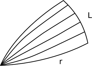
Note
In the spherical model, L = \(\rho \theta\) sin u, where u is the angle subtended at the center of the sphere by an arc of length r. We then have \(\frac{L}{L_{E}} = \frac{\sin u}{u}\), whose second derivative with respect to u is \(- \frac{1}{3}\). Since r = \(\rho\)u, the second derivative of the same quantity with respect to r equals \(− \frac{1}{3 \rho^{2}} = − \frac{K}{3}\).
Let’s now generalize beyond elliptic geometry. Consider a space modeled by a surface embedded in three dimensions, with geodesics defined as curves of extremal length, i.e., the curves made by a piece of string stretched taut across the surface. At a particular point P, we can always pick a coordinate system (x, y, z) such that the surface \(z = \frac{1}{2} k_{1} x^{2} + \frac{1}{2} k_{2} y^{2}\) locally approximates the surface to the level of precision needed in order to discuss curvature. The surface is either paraboloidal or hyperboloidal (a saddle), depending on the signs of k1 and k2. We might naively think that k1 and k2 could be independently determined by intrinsic measurements, but as we’ve seen in example 5, a cylinder is locally indistinguishable from a Euclidean plane, so if one k is zero, the other k clearly cannot be determined. In fact all that can be measured is the Gaussian curvature, which equals the product k1k2. To see why this should be true, first consider that any measure of curvature has units of inverse distance squared, and the k’s have units of inverse distance. The only possible intrinsic measures of curvature based on the k’s are therefore k21 +k22 and k1k2. (We can’t have, for example, just k21, because that would change under an extrinsic rotation about the z axis.) Only k1k2 vanishes on a cylinder, so it is the only possible intrinsic curvature.
Example 3: Eating pizza
When people eat pizza by folding the slice lengthwise, they are taking advantage of the intrinsic nature of the Gaussian curvature. Once k1 is fixed to a nonzero value, k2 can’t change without varying K, so the slice can’t droop.
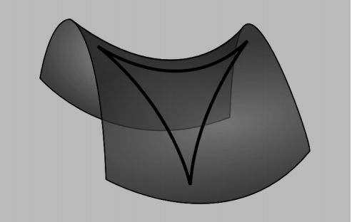
Example 4: Elliptic and hyperbolic geometry
We’ve seen that figures behaving according to the axioms of elliptic geometry can be modeled on part of a sphere, which is a surface of constant K > 0. The model can be made into global one satisfying all the axioms if the appropriate topological properties are ensured by identifying antipodal points. A paraboloidal surface z = k1x2 + k2y2 can be a good local approximation to a sphere, but for points far from its apex, K varies significantly. Elliptic geometry has no parallels; all lines meet if extended far enough.
A space of constant negative curvature has a geometry called hyperbolic, and is of some interest because it appears to be the one that describes the spatial dimensions of our universe on a cosmological scale. A hyperboloidal surface works locally as a model, but its curvature is only approximately constant; the surface of constant curvature is a horn-shaped one created by revolving a mountain-shaped curve called a tractrix about its axis. The tractrix of revolution is not as satisfactory a model as the sphere is for elliptic geometry, because lines are cut off at the cusp of the horn. Hyperbolic geometry is richer in parallels than Euclidean geometry; given a line \(\ell\) and a point P not on \(\ell\), there are infinitely many lines through P that do not pass through \(\ell\).
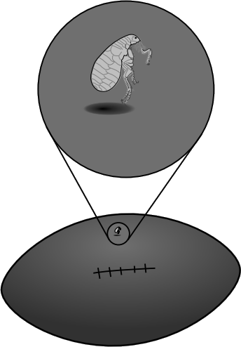
Example 5: A flea on a football
We might imagine that a flea on the surface of an American football could determine by intrinsic, local measurements which direction to go in order to get to the nearest tip. This is impossible, because the flea would have to determine a vector, and curvature cannot be a vector, since \(z = \frac{1}{2} k_{1} x^{2} + \frac{1}{2} k_{2} y^{2}\) is invariant under the parity inversion x → −x, y → −y. For similar reasons, a measure of curvature can never have odd rank.
Without violating reflection symmetry, it is still conceivable that the flea could determine the orientation of the tip-to-tip line running through his position. Surprisingly, even this is impossible. The flea can only measure the single number K, which carries no information about directions in space.
Example 6: The lightning rod
Suppose you have a pear-shaped conductor like the one in Figure 5.3.12 (1). Since the pear is a conductor, there are free charges everywhere inside it. Panels 1 and 2 of the figure show a computer simulation with 100 identical electric charges. In 1, the charges are released at random positions inside the pear. Repulsion causes them all to fly outward onto the surface and then settle down into an orderly but nonuniform pattern.
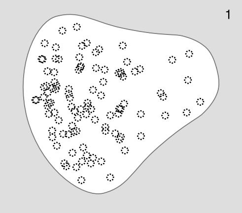
We might not have been able to guess the pattern in advance, but we can verify that some of its features make sense. For example, charge A has more neighbors on the right than on the left, which would tend to make it accelerate off to the left. But when we look at the picture as a whole, it appears reasonable that this is prevented by the larger number of more distant charges on its left than on its right.
There also seems to be a pattern to the nonuniformity: the charges collect more densely in areas like B, where the Gaussian curvature is large, and less densely in areas like C, where K is nearly zero (slightly negative).
To understand the reason for this pattern, consider Figure 5.3.12 (3). It’s straightforward to show that the density of charge \(\sigma\) on each sphere is inversely proportional to its radius, or proportional to K1/2. Lord Kelvin proved that on a conducting ellipsoid, the density of charge is proportional to the distance from the center to the tangent plane, which is equivalent3 to \(\sigma \propto\) K1/4; this result looks similar except for the different exponent. McAllister showed in 19904 that this K1/4 behavior applies to a certain class of examples, but it clearly can’t apply in all cases, since, for example, K could be negative, or we could have a deep concavity, which would form a Faraday cage. Problem 1 discusses the case of a knife-edge.
Similar reasoning shows why Benjamin Franklin used a sharp tip when he invented the lightning rod. The charged stormclouds induce positive and negative charges to move to opposite ends of the rod. At the pointed upper end of the rod, the charge tends to concentrate at the point, and this charge attracts the lightning. The same effect can sometimes be seen when a scrap of aluminum foil is inadvertently put in a microwave oven. Modern experiments5 show that although a sharp tip is best at starting a spark, a more moderate curve, like the right-hand tip of the pear in this example, is better at successfully sustaining the spark for long enough to connect a discharge to the clouds.
3 http://math.stackexchange.com/questi...f-the-distance
4 I W McAllister 1990 J. Phys. D: Appl. Phys. 23 359
5 Moore et al., Journal of Applied Meteorology 39 (1999) 593