
1.4: Gravity Lite


- Last updated
- Oct 31, 2020
- Save as PDF

( \newcommand{\kernel}{\mathrm{null}\,}\)
Puttin’ on a Little Weight
The first three chapters have talked about the consequences of the constancy of the speed of light for objects moving at uniform speeds and the observation that physics must be the same in all frames of reference. Einstein extended his theory of the constancy of the speed of light to describe situations in which acceleration was present. He called this his general theory of relativity since it contains zero acceleration (constant speed) as a limit.
Consider a spaceship undergoing constant acceleration (increasing speed) to the left in free space (far away from gravitational forces). If a beam of light enters the ship, as in the bottom picture of Figure 1.4.1a, it will hit the far wall nearer the thrusters than the point on the near wall where it entered because the ship is moving (top picture of Figure 1.4.1a).
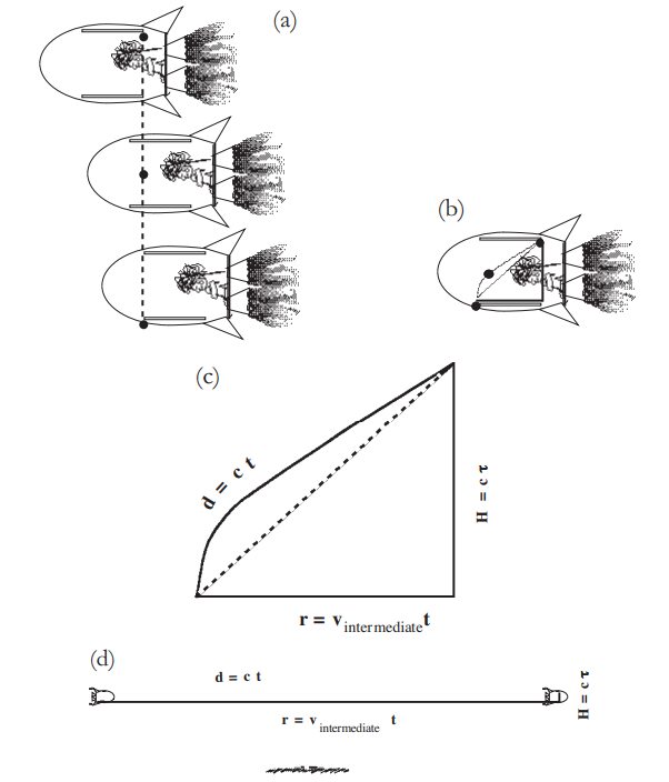
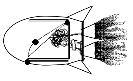
Since the ship is accelerating, its displacement relative to the beam of light increases more rapidly as time passes. For this reason, to someone sitting in the ship—such as the astronaut in Figure 1.4.1a—the beam of light will appear to bend downward, as in Figure 1.4.1b very much as if the photon of light were a ball falling in a gravitational field (projectile motion).
Had the spaceship been moving at a constant velocity intermediate between the initial and the final velocity, the path of the light would have been the hypotenuse of the triangle shown in Figure 1.4.1b and 1.4.1c. Thus, the new problem reduces to the special relativistic case when then acceleration is zero.
One can see that Figure 1.4.1c is like the pictures from chapter 1. But in the present case, with acceleration, the light path d=c t is not straight and is even longer than the hypotenuse, which you well know by now to be longer than H=c τ (where H is the distance traveled by light in the proper-time interval). You can verify this by tacking string along the curve, marking the ends of the string, and then pulling straight to get a rough measure of the length. Since c is a constant this means that, again, t is greater than τ. Thus, coordinate time is dilated relative to proper time when bodies are undergoing accelerated motion as well as when they are undergoing motion at constant velocity.
You might imagine that if the acceleration continues for a long time, or if the acceleration is very large, the shape of Figure 1.4.1c will stretch out as in Figure 1.4.1d, so much so that the curved light path will differ little from the straight hypotenuse. Both high constant speeds and large accelerations (to high speeds) give enormous time dilation.
For motion at constant velocity, we were able to graphically find the time-dilation factor by measuring the length of the hypotenuse and dividing by the length of cτ. We certainly can no longer use our rotating square since we no longer have d=c t as the hypotenuse of some triangle. But mathematics will give the correct answer.*
Note
* Even if one uses calculus to try to find this length, one must still use a simplifying approximation, in which v is much less than c, to get an algebraic expression for the result. One finds the coordinate time t and proper time τ to be related by
τ2=1+2Arc2t2,
where A is the acceleration and r is the distance moved. This is derived in the appendix.
If one properly calculates the position using the acceleration defined in terms of propertime intervals, the distance vs. coordinate time curve is a hyperbola. The distance one travels along a hyperbola, the arc-length, is not a simple expression, but a computer can draw the hyperbola corresponding to a given acceleration for you.
The Principle of Equivalence
Einstein founded his general theory of relativity on the idea that acceleration due to thrusters (Figure 1.4.2a) and gravitational acceleration (Figure 1.4.2b) must be indistinguishable since someone closed inside the spaceship would not be able to tell the difference between the two. You can prove this to yourself by finding a fast elevator in a tall building. Walk around the elevator as you start upward and you will notice that you feel very heavy. As you near your destination, also walk around the elevator and you will feel like you are on Mars.
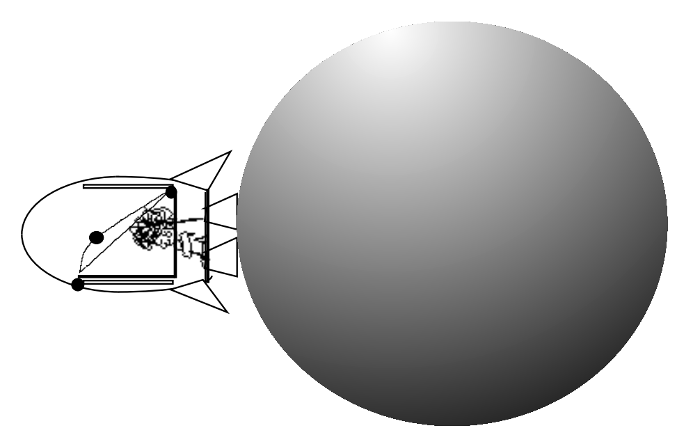
This is called the principle of equivalence. Thus, the path of a light beam near a gravitationally attractive body must be curved just as is the light beam a passenger sees passing through an accelerating spaceship.
One would like to illustrate the full four-dimensionality of this bending, but in a two-dimensional book, that is difficult to do. Artists have projected a sense of depth onto two-dimensional media by using vanishing points ever since Florentine architect Filippo Brunelleschi illustrated the Baptistery in Florence in 1415, but attempting to project four-dimensions onto two just leaves us with a mess. The solution seems to be to toss out one of the three spatial dimensions (north, west, or up), replace it with the time dimension, and project that trio onto the two dimensions of this book, as illustrated in Figure 1.4.3.
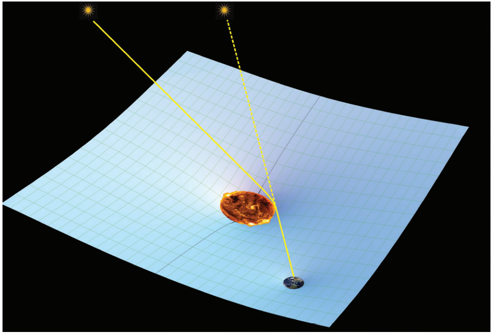
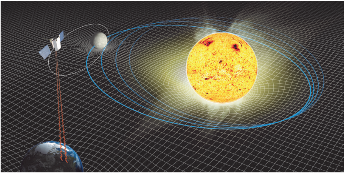
In this method, a three-dimensional scaffolding would be reduced to a two-dimensional grid, a sheet that can then be warped, like the dimple that comes of setting a bowling ball on a bed. Actually, we should reduce the bowling ball to a two-dimensional disk too, as we have done for the illustrations of the Sun and the Earth (which is causing a smaller dimple) in Figure 1.4.3. Some illustrators take the artistic license of using still-ball-shaped orbs—such as for the Sun, Mercury, and the Earth in Figure 1.4.5 —to cause such dimples in a two-dimensional space.
One final bit of license I have taken with Figure 1.4.3 is that despite declaring time to be the vertical axis in the prior paragraph, this figure appears to be frozen in time. The more complete picture would have Earth and Sun as cylinders with their upper faces moving upward, the top of which would be “now.” The light beam would be an arc upward as well as around the Sun. While this would be more correct, one can better visualize the angle through which the light beam curves by projecting the path of the light beam onto just one slice of time, which also contains a slice of the Earth and Sun cylinders at one time. This is the convention in Figures 1.4.3 and 1.4.5.
Note that a ray of light traveling through this warped spacetime must follow this warped contour. It will be bent by the warped spacetime it has to travel through. Figure 1.4.3 shows this bending in the solid yellow line. The dashed line shows the apparent position of the star as seen from Earth.
Einstein’s 1915 paper “Explanation of the Perihelion Motion of Mercury from the General Theory of Relativity” predicted that light passing close to the Sun should be bent by 1.7 seconds of arc.* On May 29, 1919, the theory was confirmed by the team of F. W. Dyson, A. S. Eddington, and C. Davidson, who measured the deflection of 12 stars during a solar eclipse and obtained values of 1.98 ± 0.16 and 1.61 ± 0.40 seconds of arc.† It was this dramatic result that brought general relativity to the attention of the general public and made Einstein a media star.
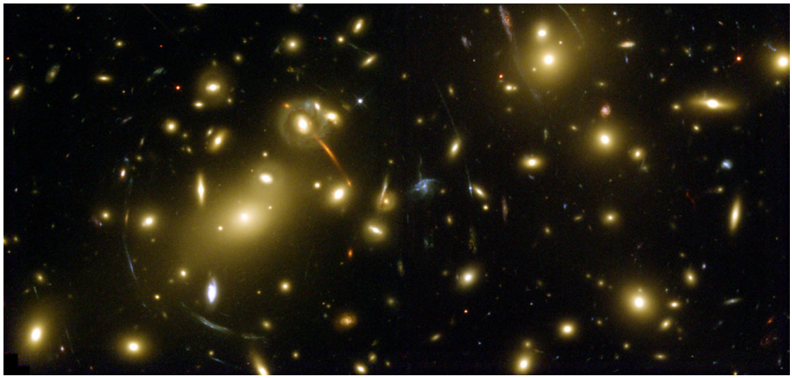
Modern telescopes reveal truly dramatic confirmations of the warping of spacetime by mass. The light from distant galaxies will be gravitationally lensed by an intervening galaxy or galactic cluster along the line of sight. This produces the arc-shaped images of the galaxy in the photograph that is Figure 1.4.4.
Note
* A. Einstein, Königlich Preußische Akademie der Wissenschaften (Berlin). Sitzungsberichte, 831–39 (November 18, 1915), https://einsteinpapers.press.princet...vol6-trans/126. There are 3,600 seconds of arc (") in a degree.
† F. W. Dyson, A. S. Eddington, and C. Davidson, Phil. Trans. Roy. Soc. 220A, 291 (1920); Mem. Roy. Astron. Soc. 62, 291 (1920).
‡ NASA, ESA, A. Fruchter, and the ERO Team (STScI, ST-ECF), The Galaxy Cluster Abell 2218, Hubble Space Telescope, https://www.spacetelescope.org/images/heic0113c/ (accessed May 7, 2020).
One other significant understanding comes from Figure 1.4.3. The warping of spacetime around the Sun is the cause of the Earth moving around the Sun rather than flying off in the straight line its momentum would otherwise produce. This is much like the orbits a coin makes in the March of Dimes funnels one finds in public spaces. In this fashion, Einstein has replaced the idea of Newton’s gravitational force with a more fundamental explanation of events that predicts the motion of light as well as massive bodies.
One may find the limit of Einstein’s equations in the case of a small warping of spacetime, such as that caused by the Sun in the vicinity of the Earth, and the results agree perfectly with Newton’s “force.” But when gravitational effects become stronger, Newton’s description becomes more and more inaccurate, whereas Einstein’s accurately predicts the state of affairs. Another key finding of Einstein’s 1915 paper was an explanation of the shift in the point of closest approach of the planet Mercury to the Sun, its perihelion. Since the 1850s astronomers had been trying to explain an anomalous extra 43 seconds of arc per century by which Mercury’s perihelion advances. In Figure 1.4.5, the blue rosette shows this advance of the perihelion, much exaggerated.
Note
* Elizabeth Zubritsky, “NASA Team Studies Middle-Aged Sun by Tracking Motion of Mercury,” National Aeronautics and Space Administration, last modified January 18, 2018, https://www.nasa.gov/feature/goddard/2018/nasa-team-studies-middle-aged-sun-by-tracking-motion-of-mercury
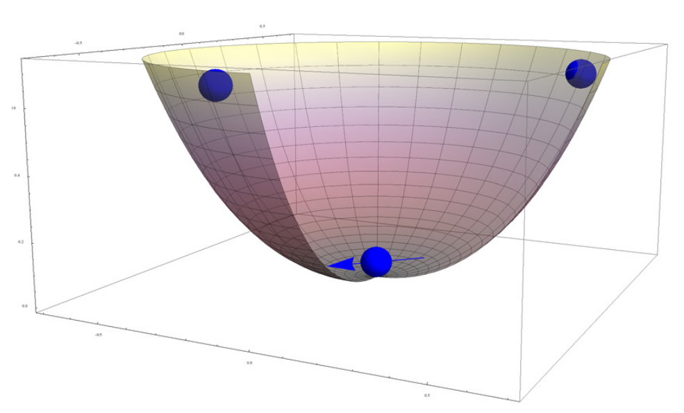
One may understand why Mercury’s perihelion advances by looking at a diagram of what is called the potential energy (PE) of its orbit. Potential energy is best understood by visualizing a marble rolling from one rim of a bowl down to the bottom, across that and up to the opposite rim, as in Figure 1.4.6. This diagram is purely Newtonian, with no “bending of spacetime” to it.
The marble is momentarily motionless at the rim so it has no kinetic energy at that point. Newton’s “gravitational force” pulls it downward, and it gains speed. It moves its fastest across the bottom of the bowl—where it has zero potential to fall further and, thus, zero potential energy—so we say that it has pure kinetic energy during that passage. It loses speed as it climbs the far wall of the bowl, converting its kinetic energy into potential energy, so that when it reaches the opposite rim, it has no kinetic energy and maximal potential energy—perhaps understood as the potential to release energy back into kinetic energy as it rolls back down.
This process is an expression of the law of conservation of energy: energy is neither created nor destroyed but simply converted from one form to another. Another example is the conversion of the stored chemical energy of gasoline into motion in a car upon combustion. Unfortunately, one cannot back up the car to get that energy back, nor will doing so retrieve the carbon the process releases into the atmosphere.
Potential energy has more utility than just helping us understand how marbles roll in physical bowls. It is an alternative way to describe a Newtonian force that causes motion. The negative of the manner in which the potential energy changes with distance is the definition of such a force. For instance, the potential energy curve for a pair of magnets whose north poles face each other looks like the left half of a U, with the horizontal position within the left half representing the closeness of the two magnets. The change in potential energy becomes more marked as one moves leftward on the left half of the U, so, by definition, the magnetic force becomes more and more repulsive as you try to bring the two north poles together. It is repulsive because the change in PE is toward more positive values, and by definition, we take the negative of this positive change to get the direction of the force. Does the force encoded in that abstract description of the PE match your visceral experience of magnets?
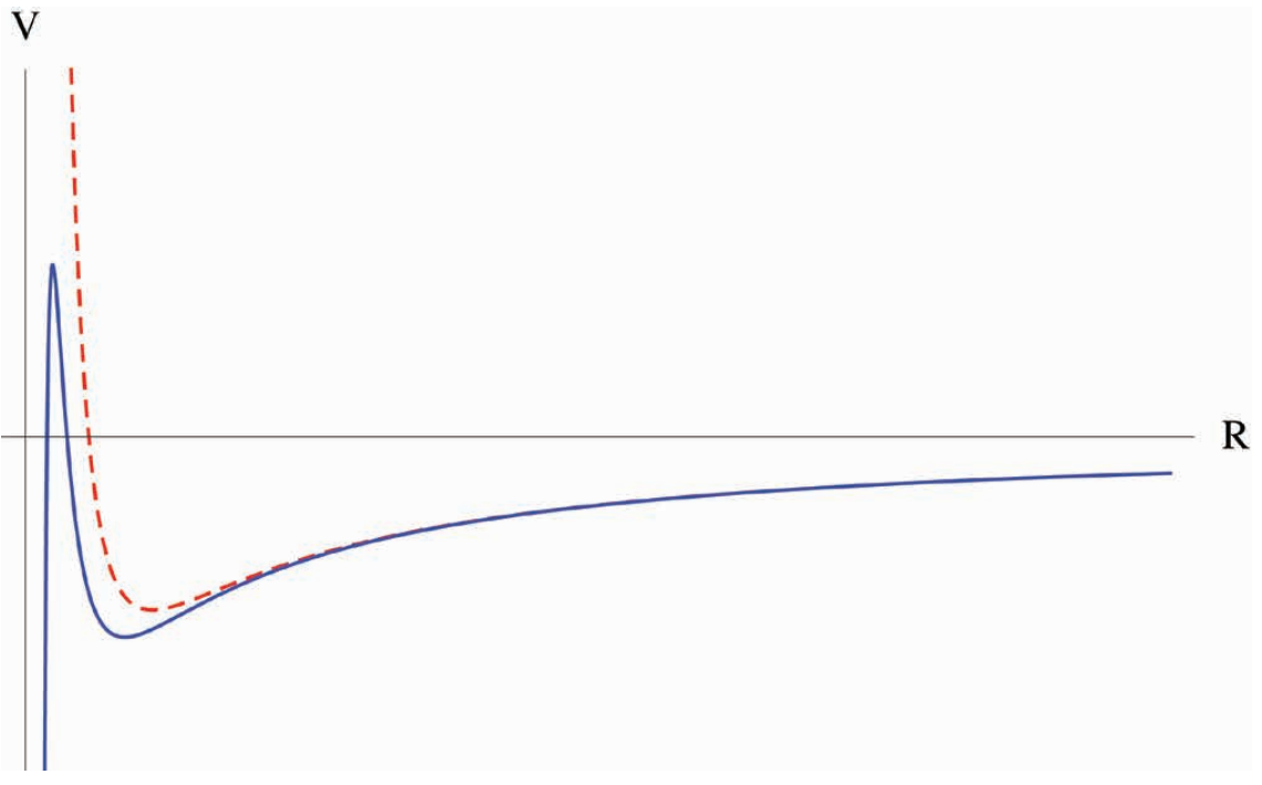
The dotted red curve in Figure 1.4.7 is a diagram of the Newtonian potential energy curve for the radius of Mercury’s orbit. One can imagine Mercury as a marble rolling back and forth in the depression. We have moved, here, from the case of a real marble rolling in a real bowl, under the influence of a real downward “Newtonian gravitational force” in Figure 1.4.6, to an abstract marble rolling in an idea, called a potential energy curve in Figure 1.4.7. In this abstract realm, it is the abstract principle that “systems seek to move to their lowest energy state” that “pulls” the marble downward; not a real downward “gravitational force” (to the extent that we can say Newtonian approximations to Einsteinian spacetime constitute a “real” gravitational force).
But what is the nature of the rim on either side of that depression? Let me ask you a couple of questions. Mercury is moving so fast that it completes one orbit in 88 days. What is it that keeps Mercury from flying off into space? In Newtonian terms, it is the tug of gravity pulling it always inward: its tendency to fly off is continually checked by the force of gravity. The energy associated with this force depends on distance as 1/R. In Einsteinian terms, the only spacetime available for Mercury to travel through is a funnel so that it is constrained to move around and around the funnel. It would need more kinetic energy to rise higher up the funnel and, hence, farther from the Sun.
What is it that keeps Mercury from falling into the Sun? Its inertia; its tendency to keep moving in a straight line unless acted upon by a force. This is the “pseudoforce” that “slams” you into the door of a car turning a corner too sharply. We call this a pseudo-force because it is really the car’s door slamming into you as it turns while you try to continue moving in a straight line. In Newtonian terms, the outward pseudoforce of inertia must be perfectly balanced by the inward gravitational force for a planet to travel in a circular orbit. If you tie a rope to a brick and swing it around your head, you must exert an inward tug on a rope to counter the outward pseudo-force of the inertia of the brick—its desire to keep moving in a straight line toward your neighbor’s window.
Consider the ice skater twirling with her arms outstretched. She will feel an outward force on her arms that her sinews must counteract. What happens when she pulls her arms in toward her body? Indeed, her spin will increase. But why is that? Just as with linear momentum, m v, which we explored in chapter 2, there is a quantity called angular momentum that is a conserved quantity. It is conventionally labeled with a script ℓ and defined as, ℓ=mvR, where R is the size of the object’s orbit. As the ice skater pulls her arms in toward her body, R becomes smaller, and in order to conserve angular momentum, v has to become larger to compensate (since m does not change). Thus, her spin will increase.
We see then that the inertia that resists the pull of sinews or the pull of a rope or the tug of gravity on a planet is closely related to angular momentum. As the skater’s arms get closer to her body, conservation of angular momentum speeds her up. As Mercury, in its elliptical orbit, gets closer to the Sun, it speeds up, and thus more effectively resists the inward pull of the stronger gravity in that region. We see that what keeps Mercury from crashing into the Sun at its closest approach is its angular momentum. That angular momentum is the left-hand “barrier” of the dotted red curve of the potential energy diagram in Figure 1.4.7. This angular momentum barrier depends on distance as 1/R2 so that it will not have much effect at large distances, where the 1/R potential energy associated with the gravitational force dominates, but it will become larger than the gravitational potential energy at small distances. To see this, divide 1 by 10 on a calculator to get 0.1. Squaring this gives 0.01, a smaller value. If you divide 1 by the larger value 100, you get a smaller result, 0.01, and squaring this gives 0.0001, a much less influential amount.
What we have done in creating Figure 1.4.7 is to fold into Mercury’s radial motion its motion around the Sun, manifesting the left-hand wall of the potential energy diagram that constrains its motion toward the Sun, keeping it from getting too close. A “marble” rolling in this potential energy diagram will therefore oscillate back and forth between the inner and outer regions, modeling the radial motion of Mercury in its orbit.
The solid blue curve in Figure 1.4.7 is the general relativistic result, which has a new term that depends in the same way on Mercury’s angular momentum as the Newtonian term. (This is one of those times when inserting lowest-order relativistic effects into a Newtonian framework pays off.) But it has a negative sign and depends on distance as 1/R3 so, at very small distances, it will dominate.
To see this, divide 1 by 0.1 on a calculator to get 10. Squaring this gives 100, the Newtonian term. Cubing your division of 1 by 0.1 gives you 1,000 as the much larger Einsteinian term. If you divide 1 by the smaller value 0.01, you get a bigger result, 100, and squaring this gives 10,000. Cubing your division of 1 by 0.01 gives you 1,000,000 as the much larger Einsteinian term. One may continue on in this fashion. The Einsteinian term will dominate when R gets small enough and, since it is negative in sign, bend the angular momentum barrier over into negative energies and incidentally moving the barrier inward.
Even for modest distance, one sees that the inward motion of a marble rolling in the Einsteinian potential energy curve is still constrained on the left, but not so strongly. The marble (Mercury) can come closer to the Sun than in the Newtonian case. It will spend more time in a region of stronger gravitational effects and will consequently have its orbit perturbed. The effect is not to make the orbit smaller or larger but to make it impossible for the orbit to close on itself. Mercury comes out of the point of closest approach shifted a bit to the side due to its penetration deeper into the Sun’s warping of spacetime. This precession of Mercury’s perihelion, which Einstein calculated in his 1915 paper to be 43 arc-seconds/century, matched the formerly unaccounted for 45 ± 5 arc-seconds/century of his day (and the more accurate 1947 value of 43.11 ± 0.45 arc-seconds/century* ), which was strong evidence in favor of his theory.
Note
* G. M. Clemence, Rev. Mod. Phys. 19, 361 (1947).
BLACK HOLES
Stars maintain their size by balancing the inward gravitational force with the outward heat pressure supplied by nuclear fusion. In the core of the star (which is under high pressure due to the outer mass of the star pressing inward), pairs of hydrogen nuclei called protons are squeezed together to form deuterons, a pair of which are then transformed into one helium nucleus, a sort of process that gives off energy. This fusion will continue for 10 billion years in a star the size of our Sun until the hydrogen in the high-pressure core is used up. For another 150 million years,* helium is fused into carbon, but there is never enough heat to fuse carbon into the heavier elements. Without these nuclear fires, the Sun will no longer have the heat pressures to maintain its present size (large enough to fit a 1.3 million Earths inside), and it will ultimately shrink to about the size of the Earth. Such a star, called a white dwarf, maintains the new size only by the quantum-mechanical pressure of electrons that do not like to occupy the same quantum state, in part their position in space. We call this quantum effect a degeneracy force.†
For a star four times more massive than our Sun, there is sufficient pressure in the core to fuse carbon into oxygen, neon, and so on until iron is produced. The star then resembles an onion with hydrogen as the outer layer and iron at the core. Once iron is produced, it is no longer possible to fuse nuclei together to form heavier elements and give off energy. So the element production stops and the star begins to shrink. For these more massive stars, the quantum mechanical electron pressure (degeneracy force) is not enough to keep the star from collapsing past the white dwarf stage. The electrons will be jammed into the protons, converting them to neutrons (and neutrinos, such as those recorded in Supernova 1987a‡), and the star collapses inward until it is about 40 km across. At this point, the neutrons stop the collapse because they, too, do not like to occupy the same region of space. This star is called a neutron star, and it is so dense that “a thimbleful of neutron-star matter brought back to Earth would weight 100 million tons.”§
In the rapid gravitational collapse, there is a rebounding of the outer layers, a shock wave that has enough extra heat and pressure to transform some of the iron into heavier elements such as zinc. Thus, the heavy elements in your body were literally produced in a stellar explosion called a supernova. One or more supernovas some 6–10 billion years ago scattered this material into the interstellar clouds of dust that eventually formed our Sun and planets. The interstellar shock wave of such explosions also helps trigger the coalescence of the solar systems out of this dust.
Note
* Eric Chaisson and Steve McMillan, Astronomy Today, 2nd ed. (Prentice Hall, Upper Saddle River, NJ, 1996), p. 428.
† For moderate-mass stars like our Sun, fusion of helium into carbon begins after the core collapses into this degenerate state. Because the pressure in this nearly degenerate gas increases only slightly with temperature (Donald D. Clayton, Principles of Stellar Evolution and Nucleosynthesis [McGraw-Hill, New York, 1968], p. 103) the core does not reexpand for hours. But the fusion rate goes up with temperature to the 40th power (R. Robert Robbins, William H. Jeffreys, and Stephen J. Shawls, Discovering Astronomy [Wiley, New York, 1995], p. 388), so the core is a runaway fusion bomb for a few hours, called a helium flash. Finally, the carbon left in the core from helium burning shrinks until electron degeneracy sets in again and, for a moderate-mass star, never gets hot enough to fuse into heavier elements.
‡ K. Hirata et al., Phys. Rev. Lett. 58, 1490 (1987).
§ That is, a density of 1014 g/cm3. William J. Kaufmann III, Discovering the Universe (W. H. Freeman, New York, 1989), p. 289.
In 1935, Subrahmanyan Chandrasekhar showed that a massive enough star that has exhausted its nuclear fuel will collapse inward, and even the quantum mechanical repulsive degeneracy force of the neutrons is insufficient to stop the star’s collapse. Such a star has no way to counter the gravitational collapse so it will continue to collapse until all the mass—of a star that was more than 100 million times bigger than the Earth—is concentrated in an area of space smaller than the smallest area you can make by holding your thumb and two fingers together. You might expect that stuffing so much mass into such a small area of space might have some pretty weird results.
Indeed, for a collapsed star, spacetime is warped infinitely deeply into the time dimension, as depicted in Figure 1.4.8. Put another way, it would take light an infinite amount of time to travel up out of this hole, and since we do not have an infinite amount of time at our disposal, we would see no light coming out. It would be black. Hence the name.
Note that a planet circling such a star before its collapse would simply continue on as if nothing had happened, aside from the inconvenience of having its atmosphere blown away in the supernova that accompanied the collapse. So black holes do not suck up everything in sight, only items on a collision course with them.
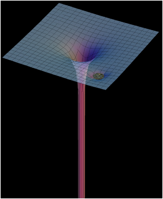
So what happens when someone starts falling down the spacetime funnel shown in Figure 1.4.8? It is intuitively obvious that they fall to the bottom and cannot get back out. Careful application of mathematics confirms this.
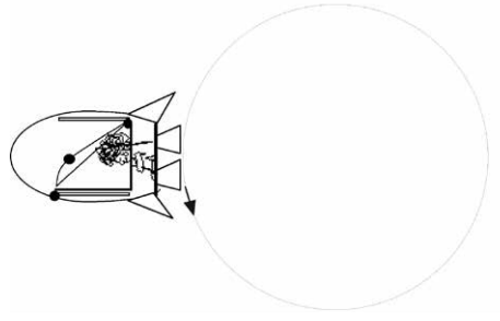
Isaac Newton showed in 1687 that the gravitational acceleration would be the same if all of a planet’s mass were concentrated at its center. Einstein said that acceleration due to thrusters and acceleration due to gravitation must be indistinguishable. So someone in a spaceship in orbit around a point-planet or collapsed star (Figure 1.4.9) encounters the same bending of light as in Figure 1.4.1a.
We wish to know how the bending of light, and the consequent time dilation, depends on closeness to a star whose mass is all contained within a point. Since gravitational acceleration increases as one gets closer, the bending, too, will increase, with a picture something like Figure 1.4.10.
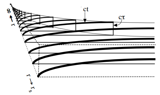
There is no bending when one is far from the star (r → ∞ at the top of Figure 1.4.10), and there is an infinite bending at the bottom as one approaches some, as yet undetermined, distance from the point in space where all the mass is concentrated. To get an intuitive sense that this distance is not zero requires some thought.
What happens if I were to throw a pen straight up? (It goes up, stops, and then falls back down.) Suppose I wanted it to go higher. What would I do? (Throw it faster.) Suppose I wanted it to travel to an infinite height before it stops and falls down again. How fast would I need to throw it?
Pretend we are on an airless planet. The easy way to find this is to use energy conservation. Actually, let us run the movie backward. Suppose we have a pen sitting at infinity and let it fall toward the Earth. How fast will it be moving just as it hits the surface? Let me just quote the result: the speed with which a pen falling from infinity would hit the Earth is
vE=√2GMRE=√2×6.67×10−11m3/s2/kg×5.95×1024kg6.378×106mvE∗=√1.24×108m2/s2=11.2km/s
Note
* The derivation is not conceptually difficult, but it is long so I put it in this footnote for the curious. Feel free to ignore it. We introduced a formal definition of the potential energy of the gravitational field when we talked about a marble rolling in a bowl (Figure 1.4.6). You can see that that marble gains kinetic energy (EK=12mv2 from chapter 2) as it moves toward the bottom of the bowl and then loses it again as it climbs the far wall.
Likewise, if we look at comets in highly elliptical orbits about the Sun, they move very fast near the Sun and slow down as they move away. They give up the potential energy that they have far from the Sun, and it is converted into kinetic energy (higher speeds) near perihelion, and that kinetic energy is converted back to potential energy as they return to the outer edges of the Solar System. The potential energy of the Earth’s gravitational field at the surface is given by
EP=−GMmr .
Why the minus sign? Well, it is convenient to define the total energy,
EK+EP=12mv2−GMmr,
as being zero at infinity (where the pen is at rest for a moment),
Ei=12m02−GMm∞=0−0=0.
Using energy conservation in this way we find that the final energy of the pen after falling from infinity will also sum to zero:
Ef=12mv2E−GMmRE=0.
Adding the same thing to both sides of an equality will not change that equality, so
12mv2E−GMmRE+GMmRE=0+GMmRE,
or
12mv2E=GMmRE.
Multiplying or dividing both sides of an equality by the same thing will not change that equality, so
2m12mv2E=2mGMmRE,
or
v2E=2GMRE.
Taking the square root of both sides of an equality will not change that equality, so
vE=√2GMRE=√2×6.67×10−11m3/s2/kg×5.95×1024kg6.378×106m.
We can run this film forward and declare that 11.2 km/s is also the speed with which we would have to throw the pen to have it escape to infinity—its escape velocity.
Now suppose all the Earth’s mass were contracted to 1/100th its size, 64,000 m. What difference would this make in these calculations? The required velocity is 10 times bigger,
v64,000m=√2GM1100RE100100=√2GMRE√100=10×11,200m/s=112,000m/s
(We are allowed to multiply any expression by one without changing its nature, and in the square root, I multiplied by a convenient form, 1 = 100/100, which helped cancel the 1/100 in the denominator by which RE was multiplied to get this compacted mass. What remains is a factor of 100 in the numerator that we then pull out of the square root.)
Suppose all the Earth’s mass were contracted to 1/100th of 1/100th its original size, 640 m. What difference would this make in these calculations?
v640 m→1,120,000m/s
Suppose all the Earth’s mass were contracted to 1/100th of that size, 6.40 m.
v6.4 m→11,200,000m/s
Suppose all the Earth’s mass were contracted to 1/100th of that size, 64 mm.
v64 mm→112,000,000m/s
Suppose all the Earth’s mass were contracted to 1/100th of that size, 0.64 mm.
v0.64 mm→1,120,000,000m/s
Do you notice anything about the size of this velocity? What is the speed of light? We’ve just exceeded it!
We had better back up and find the smallest possible size into which the Earth could be crammed so that its escape velocity would be precisely c. It turns out to be about halfway between the last two examples, 8.89 mm.
The corresponding distance at which a photon could just escape a pinpoint containing all the Sun’s mass is the ratio of masses larger:
rS=8.89mmMSME=8.89mm×333,333=2.96km
This is called the Schwarzschild radius— rs=2GMc2=2.953 km—found by Karl Schwarzschild in 1916,* a year after Einstein published his general theory of relativity.† It is fascinating to note that a dark-complected scientist and parson named John Mitchell predicted this result using Newtonian arguments in 1783.‡
Note
* K. Schwarzschild, Sitzber Deut. Akad. Wiss. Berlin, Kl. Math. Phys. Tech., 189–96 (1916); 424–34 (1916).
† The final theory appears in his fourth paper of that year: A. Einstein, Preuss. Akad. Wiss. Berlin, Sitzber., 844–47 (December 2, 1915).
‡ “The Country Parson Who Conceived of Black Holes,” American Museum of Natural History, https://www.amnh.org/ learn-teach/curriculum-collections/cosmic-horizons/case-study-john-michell-and-black-holes (accessed April 29, 2020).
GRAVITATIONAL TIME DILATION
In the section of chapter 2 entitled “The Low-Velocity Limit,” we read the Pythagorean theorem off of Figure 1.4.1, c2t2=c2τ2+v2t2, to give the exact expression for the time-dilation factor of special relativity:
γ=tτ≡1√1−v2c2
We wish to rewrite this in a pattern that will be useful for general relativity and for cosmology by squaring this and rearranging to
t2=11−v2c2τ2
For general relativity, the equivalent diagram, Figure 1.4.1c, is much more difficult to solve for the length of t relative to τ. A great deal of mathematical work to find the length of this hyperbolic curve (see the appendix) gives
t2=11−1r×2GMc2τ2
In the context of a black hole, t is the time measured by the astronaut near the Schwarzschild radius, and τ is that for an astronaut infinitely far away. The Earth-Sun distance is generally far enough away enough to give τ to good approximation.
In chapter 2, we saw that coordinate time t became infinitely dilated when v=c or, alternatively expressed, when v2=c2. If you compare the above two equations, looking for patterns as an artist might, you will notice that the position occupied by v2 in the first equation is occupied by 1r×2GM in the second equation. Since there is order in mathematics, t must become infinitely dilated when 1r×2GM=c2, or alternatively expressed, when 1c2×2GM=r. But this value of the distance is precisely the Schwarzschild radius rs=2GMc2 we just derived. What this means is that the wristwatch on an astronaut approaching the Schwarzschild radius will slow down and stop as she or he reaches the Schwarzschild radius. You may see the details in this footnote,* if you wish.
Note
* The easiest way to get meaning out of an equation is to look at its limiting values. For speeds v approaching 0, the first equation goes to
t2=11−0τ2=τ2
That is, time is not stretched. The picture that corresponds to this equation is shown in the figure here. Since c t approximately equals c τ in this picture and c is a constant, then t must approximately equal τ.
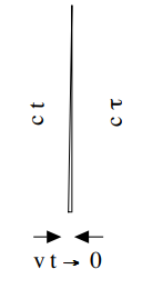
Likewise, if one goes an infinite distance from a black hole, 1/r goes to 0 in the second equation, and we have the same limiting equation above: time is not stretched. (The same limit applies if the mass M of the star is very small; there is not much spacetime warpage so we would expect the coordinate time to be about the same as proper time.)
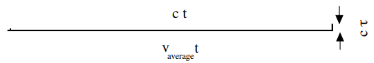
This is most easily visualized by returning to the equivalent picture of a rocket being accelerated to the left. When the acceleration is near zero, the average velocity of a rocket starting from rest is also near zero. This is shown in the second figure in this note. Far from the black hole, the gravitational bending of light is so slight that the hyperbolic path c t cannot be distinguished from the hypotenuse of the figure, which is nearly the same length as the vertical leg c τ:
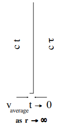
If we go to the other extreme, for speeds v approaching the speed of light, the first equation goes to
t2=11−1τ2=10τ2=∞
and coordinate time t becomes infinitely stretched compared to proper time τ as in the following picture:
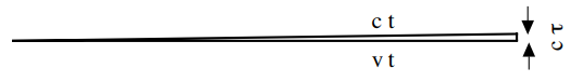
Likewise, in the case of a black hole, the second equation says that as r approaches the value rs=2GMc2, the Schwarzschild radius, the denominator again goes to 1 − 1 = 0 so that coordinate time at that radius, ts, goes to infinity. This is the place in Figure 1.4.10 where the hyperbolic path length for accelerated light c t stretches infinitely far to the right, relative to the vertical path length given by proper-time c τ that is measured at r = ∞ at the top of Figure 1.4.10. Note that in this limit also, the hyperbola is nearly superimposed over the hypotenuse of the triangle in the figure below.
Infinite gravitational time dilation happens at a finite value of r rather than at r = 0 because the speed of light is finite in the second equation, just as infinite time dilation happens at a finite value of v rather than at v = ∞ because the speed of light is finite in the first equation.
On Earth we are not infinitely far away from a gravitating body, so we cannot actually measure proper time. But all we really need anyway is a relation that compares the time dilation felt by two observers. Clearly an astronaut halfway down Figure 1.4.10 (let us call him astronaut 1) will see a wristwatch worn by an astronaut near the bottom (let us call her astronaut 2) moving at a slower rate than his own. The slower frequency will cause light coming from the whites of her eyes to look reddish to him. We say that the light is gravitationally red-shifted. On the other hand, she will see the watch worn by astronaut 1, who is further away from the star, running faster than her own. Light from the whites of this astronaut’s eyes will look bluish to her. It has been gravitationally blue-shifted.
This means that if you wear a wristwatch and an ankle watch, the latter will literally run more slowly than the former. Since your ankle is only 1 m closer to the center of the Earth (6,378,000 m away) than is your wrist, and the mass of the Earth is relatively small, the difference is only 1 part in 5,000,000,000,000,000.* That is, you will age faster by one microsecond for every story (3 m) higher you live above the surface of the Earth.
The closer astronaut 2 gets to the black hole, the slower her watch will appear to run to astronaut 1. In fact, it would take an infinite amount of 1’s time for a second to pass on 2’s watch as she just approaches rs. Also, the closer she gets, the redder the light from the whites of her eyes will appear, passing in turn through red, infrared, microwave, and radio wavelengths until the wavelength would be so long as to be undetectable. Thus, we find that light cannot get out of the region inside rs, and that is why we call an object with such a singularity in free space a black hole. Likewise, as astronaut 2 gets closer to the Schwarzschild radius, she sees the clocks on the spaceship far from the black hole carrying astronaut 1 spin faster. In fact, while 2 is having lunch, she would see that billions of years pass in the outside universe. The whites of astronaut 1’s eyes will become bluish, then give off ultraviolet radiation, then X-rays, and then gamma rays. Fortunately, her cone of observation simultaneously closes up so that the amount of this harsh radiation reaching astronaut 2 is diminished enough for her to survive it.
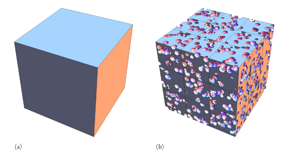
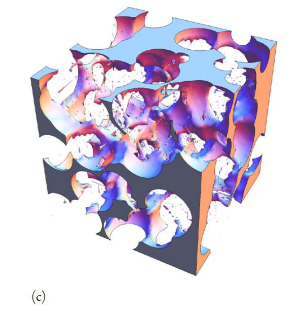
The biggest problem for astronaut 2 to worry about after lunch is that she will crash into, and become part of, the singularity at r = 0, the place where all the star’s mass is concentrated. Einstein’s classical theory of gravity says that as she approached the singularity, it would have such a strong tidal effect that our poor astronaut would be stretched out to an infinite extent. However, quantum mechanics tells us that spacetime loses its smoothness as one experiences distances as small relative to the size of a proton as the proton is to us. Moving through distances this near the origin requires quantum jumps from one piece of a sponge-like space to another, as in Figure 1.4.11c, a state of affairs not contained in Einstein’s classical theory of gravity.
Note
* We can use the second equation twice to find the algebraic expression that represents this concept. If we say that observer 1 is at distance a r1 from the star and observer 2 is at distance r2 from the star. Then the coordinate times are related by t1=√1−2GM/r1c2√1−2GM/r2c2t2. Because the Earth’s mass is small, this is approximately equal to t1≅[1−2GMr2c2(r1−r2)r1]t2=[1−2.18×10⁻¹⁶]t2.
The red-shifting of light can be detected in light emitted from the surface of our Sun and seen on the Earth. If we had sensitive enough instruments to measure it, light coming from the surface of the Moon would be blue-shifted when seen on the Earth’s surface.
We do not yet have a coherent quantum theory of gravity, but hybrid quantum calculations tell us that near r = 0, for a newly collapsed star, our astronaut would actually be folded back and forth like a piece of taffy.* An astronaut who waits until the hole is many years old before taking the plunge will face “tidal forces surrounding the singularity . . . so tame and meek, according to [Werner] Israel’s, [Eric] Poisson’s,† and [Amos] Ori’s [1991] calculations,‡ that the astronaut will hardly feel them at all. [Sh]e will survive, almost unscathed, right up to the edge of the probabilistic quantum gravity singularity. Only at the singularity’s edge, just as [s]he comes face-to-face with the laws of quantum gravity, will the astronaut be killed—and we cannot even be absolutely sure [s]he gets killed then, since we do not really understand at all well the laws of quantum gravity and their consequences.”§
Note
* Kip S. Thorne, From Black Holes to Time Warps: Einstein’s Outrageous Legacy (W. W. Norton, New York, 1994), p. 474.
† W. Israel and E. Poisson, Phys. Rev. D 41, 1796 (1990).
‡ A. Ori, Phys. Rev. Lett. 67, 789 (1991).
§ Kip S. Thorne, From Black Holes to Time Warps: Einstein’s Outrageous Legacy (W. W. Norton, New York, 1994), p. 479.
There may even be a way to avoid a singularity completely. If the collapsing star were spinning, it would collapse onto a ring of no thickness (whose radius increases with the ratio of the rotational velocity to the mass of the black hole‡) rather than a point of no thickness.§ In fact, it’s very unlikely that a star would form with zero spin, or lose its spin as it collapses, so these Kerr black holes,¶ with their ring singularity, would be the norm. Our astronaut could conceivably pass through the center of the ring and miss the singularity. But then what?
Note
‡ Robert M. Wald, General Relativity (University of Chicago Press, Chicago, 1984), p. 314–15, gives the ring singularity at r=GJMc3, where J is the total angular momentum of the collapsed star and its gravitational field (Steven Weinberg, Gravitation and Cosmology: Principles and Applications of the General Theory of Relativity [Wiley, New York, 1972], p. 240) and G is the gravitational constant.
§ For a spinning Kerr black hole, the surface of infinite time dilation and the one-way membrane are two different ellipsoidal surfaces,
.PNG?revision=1&size=bestfit&width=214&height=169)
whereas for a nonspinning black hole, these are combined into the spherical shell at the Schwarzschild radius. We will see infinite time dilation for an astronaut passing through the outermost ellipsoid of revolution, r+, but she could reemerge from this surface. The inner ellipsoid of revolution, r−, is the one-way surface of the Kerr black hole. Once she passes through r−, our astronaut is lost to us. But interestingly, maybe not lost to herself. See Ronald Adler, Maurice Bazin, and Menachem Schriffer, Introduction to General Relativity (McGraw-Hill, New York, 1975), p. 265.
¶ Roy P. Kerr, Phys. Rev. Lett. 11, 237–38 (1963).
Einstein’s equations allow a solution in which our astronaut would pass through the ring into a region called a white hole because time is reversed there so everything near the ring singularity travels out of a different one-way membrane into a flat region of our universe other than the one it started in or into another universe. I emphasized the word “allow” because one would actually have to “start” with the two flat regions of spacetime connected by a singularity so that the collapse of a star is unlikely to lead to such a wormhole.** No white hole has ever been seen.
Note
** Robert M. Wald, General Relativity (University of Chicago Press, Chicago, 1984), p. 155.
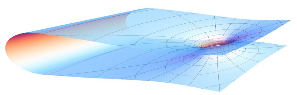
Supposing such a wormhole is found, and our astronaut falls in, appearing redder and redder and seeming to take forever to do so to the outside world. She looks out and sees the outside universe appearing bluer and bluer and watches their clocks speed up. She sees an inconceivable number of years pass outside while it takes a few minutes of her time for her to pass through the wormhole into some other part of the same universe she left, in the distant future, or perhaps into another universe. Figure 1.4.12 shows a wormhole connecting two regions of the same universe. With only two spatial dimensions shown, one is free to imagine the space portion bent around a curve in the time dimension and back the way it came. Thus, a trip that would take the spaceship eons by traveling leftward through space on the lower two-dimensional sheet—from a star near the wormhole, up around the curve, and back rightward—toward another star near the other end of the wormhole on the upper two-dimensional sheet could, in principle, be accomplished in much less time by traveling through the wormhole to the other two-dimensional spatial sheet, with the two openings of the wormhole separated by a time interval. The wormhole thus connects two very distant spatial places.
Unfortunately, this would appear to be a one-way trip. Going back through would put her further into the future. So even if we had some brave volunteers to test these hypotheses, we would never know the answer.
GRAVITATIONAL WAVES
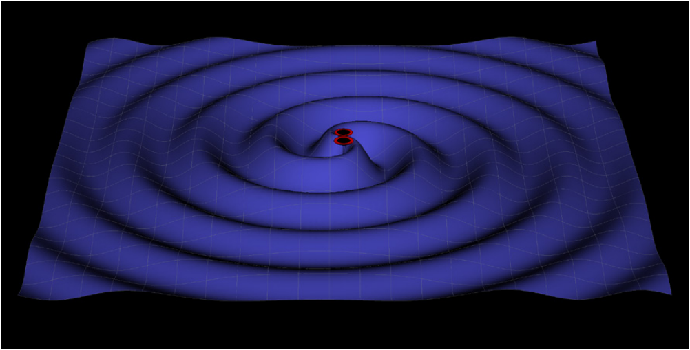
In 1916, Einstein predicted that the motion of massive objects would cause spacetime ripples, or gravitational waves. Figure 1.4.13 shows a pair of black holes orbiting each other, and their stirring of spacetime locally sends out an expanding ripple of gravitational waves.
The first clue that gravitational waves might be real was Russell Hulse and Joseph Taylor Jr.’s 1975 discovery of a pulsar orbiting a neutron star that was slowing down, apparently due to the emission of gravitational radiation waves,† work that later earned them the 1993 Nobel Prize. As the pulsar and neutron star lose energy via gravitational waves, they spiral inward over billions of years and will eventually crash into each other.
Explicit confirmation of the existence of gravitational waves from such a source came on September 14, 2015, thanks to the twin Laser Interferometer Gravitational-Wave Observatory (LIGO) detectors located in Livingston, Louisiana, and Hanford, Washington, which each detected a passing gravitational wave. Figure 1.4.14 shows the characteristic sound of spacetime ringing as two black holes collide. In this final fraction of a second, the two black holes collide at nearly half the speed of light to form a single black hole and convert some of the mass of the black holes into wave energy. Only this peak energy is strong enough for LIGO to detect.
The signals came from two merging black holes lying 1.3 billion light-years away, one about 29 solar masses (29 times the mass of our Sun) and the other about 36 solar masses. The final, merged black hole was 62 times heavier than the Sun, and the remaining 3 solar masses were emitted as the energy of the massive gravitational wave crest that was detected.
Note
* Modified from a Mathematica notebook by Jeff Bryant at https://community.wolfram.com/groups/-/m/t/790989. He notes, “The function being plotted is not derived from any general relativity equations. It’s a very similar surface to the one used on the Wikipedia page for eLISA, and in fact was designed to try to emulate this.”
† R. A. Hulse and J. H. Taylor, Ap. J. 195, L51 (1975).
On December 26, 2015, a second merger was detected from a pair of black holes 1.4 billion light-years away and which had about 14.2 and 7.5 times the mass of the Sun.
The 2017 Nobel Prize in Physics was awarded to three key figures in the development and success of LIGO: Barry Barish, Kip Thorne, and Rainer Weiss.
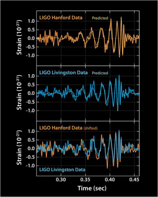
Figure 1.4.14: The signals of gravitational waves detected by the twin LIGO observatories at Livingston, Louisiana, and Hanford, Washington, from the merger of two black holes. The top signal at Hanford arrived 1/7000th of a second after the signal first reached Livingston, the middle plot, which shows that it traveled at the speed of light. The bottom plot compares data from both detectors, with the Hanford data shifted by that time interval and inverted to account for the different orientation of the detectors at the two sites.
The signals, including the instruments’ ever-present noise, were compared against numerous simulated signals, based on the equations of general relativity, varying by mass and distance. The best fit was for a merger of two black holes—one about 29 times the mass of the Sun and the other about 36 solar masses—lying 1.3 billion light-years away. This comparison is shown in white. Time is plotted on the x-axis and strain on the y-axis. Strain represents the fractional amount by which distances are distorted—less than the width of a proton. Image credit: Caltech / MIT / LIGO Lab.*
Note
* “Gravitational Waves, as Einstein Predicted,” LIGO Laboratory, https://www.ligo.caltech.edu/image/ligo20160211a (accessed May 7, 2020).