5.11: Manifolds (Part 1)

This section can be omitted on a first reading.

Why We Need Manifolds

General relativity doesn’t assume a predefined background metric, and this creates a chicken-and-egg problem. We want to define a metric on some space, but how do we even specify the set of points that make up that space? The usual way to define a set of points would be by their coordinates. For example, in two dimensions we could define the space as the set of all ordered pairs of real numbers (x, y). But this doesn’t work in general relativity, because space is not guaranteed to have this structure. For example, in the classic 1979 computer game Asteroids, space “wraps around,” so that if your spaceship flies off the right edge of the screen, it reappears on the left, and similarly at the top and bottom (Figure \(\PageIndex{1}\)).

Figure \(\PageIndex{1}\): In Asteroids, space “wraps around.”

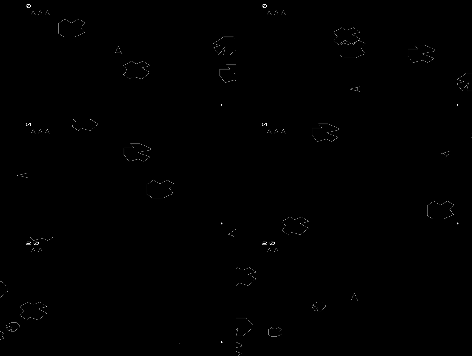
Even before we impose a metric on this space, it has topological properties that differ from those of the Euclidean plane. By “topological” we mean properties that are preserved if the space is thought of as a sheet of rubber that can be stretched in any way, but not cut or glued back together. Topologically, the space in Asteroids is equivalent to a torus (surface of a doughnut), but not to the Euclidean plane.

Figure \(\PageIndex{2}\): A coffee cup is topologically equivalent to a torus.

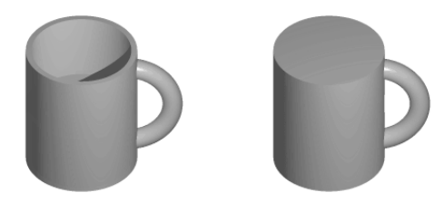
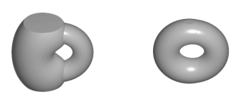
Another useful example is the surface of a sphere. In example 10, we calculated \(\Gamma^{\theta}_{\phi \phi}\). A similar calculation gives \(\Gamma^{\theta}_{\phi \phi} = \cot \frac{\theta}{R}\). Now consider what happens as we drive our dogsled north along the line of longitude \(\phi\) = 0, cross the north pole at \(\theta\) = 0, and continue along the same geodesic. As we cross the pole, our longitude changes discontinuously from 0 to \(\pi\). Consulting the geodesic equation, we see that this happens because \(\Gamma^{\theta}_{\phi \phi}\) blows up at \(\theta\) = 0. Of course nothing really special happens at the pole. The bad behavior isn’t the fault of the sphere, it’s the fault of the \((\theta, \phi)\) coordinates we’ve chosen, that happen to misbehave at the pole. Unfortunately, it is impossible to define a pair of coordinates on a two-sphere without having them misbehave somewhere. (This follows from Brouwer’s famous 1912 “Hairy ball theorem,” which states that it is impossible to comb the hair on a sphere without creating a cowlick somewhere.)

Topological Definition of a Manifold

This motivates us to try to define a “bare-bones” geometrical space in which there is no predefined metric or even any predefined set of coordinates.

There is a general notion of a topological space, which is too general for our purposes. In such a space, the only structure we are guaranteed is that certain sets are defined as “open,” in the same sense that an interval like 0 < x < 1 is called “open.” A point in an open set can be moved in any direction without leaving the set. An open set is essentially a set without a boundary, for in a set like 0 ≤ x ≤ 1, the boundary points 0 and 1 can only be moved in one direction without taking them outside.

Figure \(\PageIndex{3}\): General relativity does not assume a predefined background metric. Therefore all we can really know before we calculate anything is that we’re working on a manifold, without a metric imposed on it.

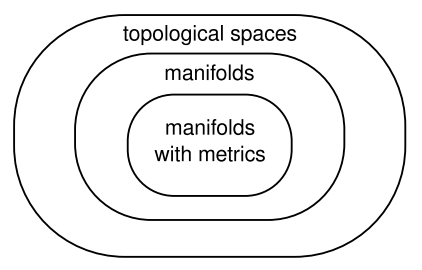
A topological space is too general for us because it can include spaces like fractals, infinite-dimensional spaces, and spaces that have different numbers of dimensions in different regions. It is nevertheless useful to recognize certain concepts that can be defined using only the generic apparatus of a topological space, so that we know they do not depend in any way on the presence of a metric. An open set surrounding a point is called a neighborhood of that point. In a topological space we have a notion of getting arbitrarily close to a certain point, which means to take smaller and smaller neighborhoods, each of which is a subset of the last. But since there is no metric, we do not have any concept of comparing distances of distant points, e.g., that P is closer to Q than R is to S. A continuous function is a purely topological idea; a continuous function is one such that for any open subset U of its range, the set V of points in its domain that are mapped to points in U is also open. Although some definitions of continuous functions talk about real numbers like \(\epsilon\) and \(\delta\), the notion of continuity doesn’t depend on the existence of any structure such as the real number system. A homeomorphism is a function that is invertible and continuous in both directions. Homeomorphisms formalize the informal notion of “rubber-sheet geometry without cutting or gluing.” If a homeomorphism exists between two topological spaces, we say that they are homeomorphic; they have the same structure and are in some sense the same space.

The more specific type of topological space we want is called a manifold. Without attempting any high level of mathematical rigor, we define an n-dimensional manifold M according to the following informal principles:¹⁶

Note

For those with knowledge of topology, these can be formalized a little more: we want a completely normal, second-countable, locally connected topological space that has Lebesgue covering dimension n, is a homogeneous space under its own homeomorphism group, and is a complete uniform space. I don’t know whether this is sufficient to characterize a manifold completely, but it suffices to rule out all the counterexamples of which I know.

• M1 Dimension: M’s dimension is n.
• M2 Homogeneity: No point has any locally definable property that distinguishes it from any other point.
• M3 Completeness: M is complete, in the sense that specifying an arbitrarily small neighborhood gives a unique definition of a point.

Example 12: Lines

The set of all real numbers is a 1-manifold. Similarly, any line with the properties specified in Euclid’s Elements is a 1-manifold. All such lines are homeomorphic to one another, and we can therefore speak of “the line.”

Example 13: a circle

A circle (not including its interior) is a 1-manifold, and it is not homeomorphic to the line. To see this, note that deleting a point from a circle leaves it in one connected piece, but deleting a point from a line makes two. Here we use the fact that a homeomorphism is guaranteed to preserve “rubber-sheet” properties like the number of pieces.

Example 14: No changes of dimension

A “lollipop” formed by gluing an open 2-circle (i.e., a circle not including its boundary) to an open line segment is not a manifold, because there is no n for which it satisfies M1.

It also violates M2, because points in this set fall into three distinct classes: classes that live in 2-dimensional neighborhoods, those that live in 1-dimensional neighborhoods, and the point where the line segment intersects the boundary of the circle.

Example 15: No manifolds made from the rational numbers

The rational numbers are not a manifold, because specifying an arbitrarily small neighborhood around \(\sqrt{2}\) excludes every rational number, violating M3.

Similarly, the rational plane defined by rational-number coordinate pairs (x, y) is not a 2-manifold. It’s good that we’ve excluded this space, because it has the unphysical property that curves can cross without having a point in common. For example, the curve y = x² crosses from one side of the line y = 2 to the other, but never intersects it. This is physically undesirable because it doesn’t match up with what we have in mind when we talk about collisions between particles as intersections of their world-lines, or when we say that electric field lines aren’t supposed to intersect.

Example 16: no boundary

The open half-plane y > 0 in the Cartesian plane is a 2-manifold. The closed half-plane y ≥ 0 is not, because it violates M2; the boundary points have different properties than the ones on the interior.

Example 17: Disconnected manifolds

Two nonintersecting lines are a 1-manifold. Physically, disconnected manifolds of this type would represent a universe in which an observer in one region would never be able to find out about the existence of the other region.

Example 18: No bad glue jobs

Hold your hands like you’re pretending you know karate, and then use one hand to karate-chop the other. Suppose we want to join two open half-planes in this way. As long as they’re separate, then we have a perfectly legitimate disconnected manifold. But if we want to join them by adding the point P where their boundaries coincide, then we violate M2, because this point has special properties not possessed by any others. An example of such a property is that there exist points Q and R such that every continuous curve joining them passes through P. (Cf. problem 5)

Hausdorff Property

Pioneering topologist Felix Hausdorff defined the following property of a topological space.

Definition: Hausdorff property

Given any two points, it is possible to find disjoint neighborhoods of them.

A joke/mnemonic, which probably works best for people with a certain type of British accent, is that in a Hausdorff space, any two points can be “housed off” from one another inside their own nonintersecting open sets. The notion appeals strongly to our intuitive ideas about how space and time behave, and the standard definition of a manifold implies that it is Hausdorff. When we model Minkowski space using real-number coordinates, it is Hausdorff. Since the equivalence principle says that spacetime is locally Minkowski, we could also say that it implies spacetime is Hausdorff. However, general relativity allows spacetime to behave badly in cases such as singularities, so it is imaginable that our universe contains points that violate the Hausdorff property. There are interesting and physically well-motivated spacetimes, such as some versions of the Taub-NUT space, that are non-Hausdorff. Since we have no empirical data on the behavior of spacetime under the most extreme conditions, we cannot say whether spacetime is really Hausdorff. One should maintain some skepticism about whether such an idealized category is even meaningful in science, since it refers to phenomena at arbitrarily small scales, whereas theories and measurements are limited in the scales they can deal with. A good discussion of the Hausdorff property as applied to relativity is given by Earman.¹⁷

Example 19: Branching universes

Figure \(\PageIndex{4}\) shows spacetime diagrams of 1 + 1-dimensional universes that branch like a tree. These are meant to be pictures of classical general relativity, although some of the strongest motivation for considering such possibilities comes from attempts to construct a theory of quantum gravity. In such theories, it is commonly expected that spacetime will have a structure at the Planck scale that is a kind of “quantum foam.”

Figure \(\PageIndex{4}\): Spacetime diagrams of 1 + 1-dimensional universes.

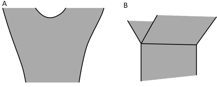
The example in Figure \(\PageIndex{4A}\) is a manifold, and is Hausdorff. This is an example of topology change, meaning that the spacelike section at one time has a different topology than the section at another.¹⁸ Although such a branching can occur without the existence of any singularities, theorems by Tipler and Geroch show that other types of misbehavior must occur, including causality violations and the need for forms of matter that violate energy conditions.

Figure \(\PageIndex{4B}\) is qualitatively different. Here we have formed a spacetime by gluing together three pieces. No curvature is implied; these could be three pieces of Minkowski space. The spacetime is not a manifold, since the points at the join have different local properties than points elsewhere. The machinery of general relativity breaks down in a case like this, but for example we could imagine that a geodesic in this spacetime could fork off into two different geodesics after the split.

Yet a third possibility is to reinterpret Figure \(\PageIndex{4B}\) so that there are two different copies of the seam. For example, we could let the portion of the diagram extending into the past be represented by points with t < 0, while the two branches continuing into the future could each have t ≥ 0, so that for a given x we would have two different events with coordinates (t = 0, x). It would not be possible to put these two points into disjoint neighborhoods, so this version of the space is not Hausdorff.

---

¹⁸ For a recent treatment, see Borde, 1994, “Topology change in classical general relativity,” arxiv.org/abs/gr-qc/9406053.

References

¹⁷ John Earman, ‘Pruning some branches from “branching spacetimes”,’ pitt.edu/~jearman/Earman2008a.pdf