5.9: Torsion

This section describes the concept of gravitational torsion. It can be skipped without loss of continuity, provided that you accept the symmetry property \(\Gamma^{a}_{[bc]} = 0\) without worrying about what it means physically or what empirical evidence supports it.

Exercise \(\PageIndex{1}\)

Self-check: Interpret the mathematical meaning of the equation \(\Gamma^{a}_{[bc]} = 0\), which is expressed in the notation introduced earlier.

Are Scalars Path-dependent?

It seems clear that something like the covariant derivative is needed for vectors, since they have a direction in spacetime, and thus their measures vary when the measure of spacetime itself varies. Since scalars don’t have a direction in spacetime, the same reasoning doesn’t apply to them, and this is reflected in our rules for covariant derivatives. The covariant derivative has one \(\Gamma\) term for every index of the tensor being differentiated, so for a scalar there should be no \(\Gamma\) terms at all, i.e., \(\nabla_{a}\) is the same as \(\partial_{a}\).

But just because derivatives of scalars don’t require special treatment for this particular reason, that doesn’t mean they are guaranteed to behave as we intuitively expect, in the strange world of coordinate-invariant relativity.

One possible way for scalars to behave counterintuitively would be by analogy with parallel transport of vectors. If we stick a vector in a box (as with, e.g., the gyroscopes aboard Gravity Probe B) and carry it around a closed loop, it changes. Could the same happen with a scalar? This is extremely counterintuitive, since there is no reason to imagine such an effect in any of the models we’ve constructed of curved spaces. In fact, it is not just counterintuitive but mathematically impossible, according to the following argument. The only reason we can interpret the vector-in-a-box effect as arising from the geometry of spacetime is that it applies equally to all vectors. If, for example, it only applied to the magnetic polarization vectors of ferromagnetic substances, then we would interpret it as a magnetic field living in spacetime, not a property of spacetime itself. If the value of a scalar-in-a-box was path-dependent, and this path-dependence was a geometric property of spacetime, then it would have to apply to all scalars, including, say, masses and charges of particles. Thus if an electron’s mass increased by 1% when transported in a box along a certain path, its charge would have to increase by 1% as well. But then its charge-to-mass ratio would remain invariant, and this is a contradiction, since the charge-to-mass ratio is also a scalar, and should have felt the same 1% effect. Since the varying scalar-in-a-box idea leads to a contradiction, it wasn’t a coincidence that we couldn’t find a model that produced such an effect; a theory that lacks self-consistency doesn’t have any models.

Exercise \(\PageIndex{2}\)

Self-check: Explain why parallel transporting a vector can only rotate it, not change its magnitude.

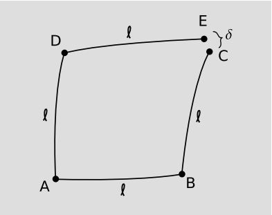
There is, however, a different way in which scalars could behave counterintuitively, and this one is mathematically self-consistent. Suppose that Helen lives in two spatial dimensions and owns a thermometer. She wants to measure the spatial variation of temperature, in particular its mixed second derivative \(\frac{\partial^{2} T}{\partial x \partial y}\). At home in the morning at point A, she prepares by calibrating her gyrocompass to point north and measuring the temperature. Then she travels \(\ell\) = 1 km east along a geodesic to B, consults her gyrocompass, and turns north. She continues one kilometer north to C, samples the change in temperature \(\Delta T_{1}\) relative to her home, and then retraces her steps to come home for lunch. In the afternoon, she checks her work by carrying out the same process, but this time she interchanges the roles of north and east, traveling along ADE. If she were living in a flat space, this would form the other two sides of a square, and her afternoon temperature sample \(\Delta T_{2}\) would be at the same point in space C as her morning sample. She actually doesn’t recognize the landscape, so the sample points C and E are different, but this just confirms what she already knew: the space isn’t flat.¹⁰

Figure \(\PageIndex{1}\) - Measuring \(\frac{\partial^{2} T}{\partial x \partial y}\) for a scalar T.

Figure \(\PageIndex{2}\) - The gyroscopes both rotate when transported from A to B, causing Helen to navigate along BC, which does not form a right angle with AB. The angle between the two gyroscopes’ axes is always the same, so the rotation is not locally observable, but it does produce an observable gap between C and E.

Note

This point was mentioned in section 5.4, in connection with the definition of the Riemann tensor.

None of this seems surprising yet, but there are now two qualitatively different ways that her analysis of her data could turn out, indicating qualitatively different things about the laws of physics in her universe. The definition of the derivative as a limit requires that she repeat the experiment at smaller scales. As \(\ell\) → 0, the result for \(\frac{\partial^{2} T}{\partial x \partial y}\) should approach a definite limit, and the error should diminish in proportion to \(\ell\). In particular the difference between the results inferred from \(\Delta T_{1}\) and \(\Delta T_{2}\) indicate an error, and the discrepancy between the second derivatives inferred from them should shrink appropriately as \(\ell\) shrinks. Suppose this doesn’t happen. Since partial derivatives commute, we conclude that her measuring procedure is not the same as a partial derivative. Let’s call her measuring procedure \(\nabla\), so that she is observing a discrepancy between \(\nabla_{x} \nabla_{y}\) and \(\nabla_{y} \nabla_{x}\). The fact that the commutator \(\nabla_{x} \nabla_{y} − \nabla_{y} \nabla_{x}\) doesn’t vanish cannot be explained by the Christoffel symbols, because what she’s differentiating is a scalar. Since the discrepancy arises entirely from the failure of \(\Delta T_{1} − \Delta T_{2}\) to scale down appropriately, the conclusion is that the distance \(\delta\) between the two sampling points is not scaling down as quickly as we expect. In our familiar models of two-dimensional spaces as surfaces embedded in three-space, we always have \(\delta \sim \ell^{3}\) for small \(\ell\), but she has found that it only shrinks as quickly as \(\ell^{2}\).

For a clue as to what is going on, note that the commutator \(\nabla_{x} \nabla_{y} − \nabla_{y} \nabla_{x}\) has a particular handedness to it. For example, it flips its sign under a reflection across the line y = x. When we “parallel”-transport vectors, they aren’t actually staying parallel. In this hypothetical universe, a vector in a box transported by a small distance \(\ell\) rotates by an angle proportional to \(\ell\). This effect is called torsion. Although no torsion effect shows up in our familiar models, that is not because torsion lacks self-consistency. Models of spaces with torsion do exist. In particular, we can see that torsion doesn’t lead to the same kind of logical contradiction as the varying-scalar-in-a-box idea. Since all vectors twist by the same amount when transported, inner products are preserved, so it is not possible to put two vectors in one box and get the scalar-in-a-box paradox by watching their inner product change when the box is transported.

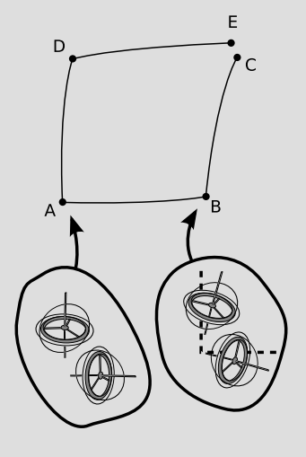
Note that the elbows ABC and ADE are not right angles. If Helen had brought a pair of gyrocompasses with her, one for x and one for y, she would have found that the right angle between the gyrocompasses was preserved under parallel transport, but that a gyrocompass initially tangent to a geodesic did not remain so. There are in fact two inequivalent definitions of a geodesic in a space with torsion. The shortest path between two points is not necessarily the same as the straightest possible path, i.e., the one that parallel-transports its own tangent vector.

The Torsion Tensor

Since torsion is odd under parity, it must be represented by an odd-rank tensor, which we call \(\tau^{c}_{ab}\) and define according to

\[(\nabla_{a} \nabla_{b} - \nabla_{b} \nabla_{a})f = - \tau^{c}_{ab} \nabla_{c} f,\]

where f is any scalar field, such as the temperature in the preceding section. There are two different ways in which a space can be non-Euclidean: it can have curvature, or it can have torsion. For a full discussion of how to handle the mathematics of a spacetime with both curvature and torsion, see the article by Steuard Jensen at http://www.slimy.com/~steuard/teaching/tutorials/GRtorsion.pdf. For our present purposes, the main mathematical fact worth noting is that vanishing torsion is equivalent to the symmetry \(\Gamma^{a}_{bc} = \Gamma^{a}_{cb}\) of the Christoffel symbols. Using the notation introduced earlier, \(\Gamma^{a}_{[bc]} = 0\) if \(\tau = 0\).

Exercise \(\PageIndex{3}\)

Self-check: Use an argument similar to the one in example 5 to prove that no model of a two-space embedded in a three-space can have torsion.

Generalizing to more dimensions, the torsion tensor is odd under the full spacetime reflection x_a → −x_a, i.e., a parity inversion plus a time-reversal, PT.

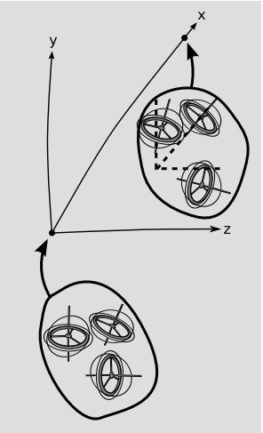
In the story above, we had a torsion that didn’t preserve tangent vectors. In three or more dimensions, however, it is possible to have torsion that does preserve tangent vectors. For example, transporting a vector along the x axis could cause only a rotation in the y-z plane. This relates to the symmetries of the torsion tensor, which for convenience we’ll write in an x-y-z coordinate system and in the fully covariant form \(\tau_{\lambda \mu \nu}\). The definition of the torsion tensor implies \(\tau_{\lambda (\mu \nu)} = 0\), i.e., that the torsion tensor is antisymmetric in its two final indices. Torsion that does not preserve tangent vectors will have nonvanishing elements such as \(\tau_{xxy}\), meaning that parallel-transporting a vector along the x axis can change its x component. Torsion that preserves tangent vectors will have vanishing \(\tau_{\lambda \mu \nu}\) unless \(\lambda, \mu\), and \(\nu\) are all distinct. This is an example of the type of antisymmetry that is familiar from the vector cross product, in which the cross products of the basis vectors behave as x × y = z, y × z = x, y × z = x. Generalizing the notation for symmetrization and antisymmetrization of tensors from earlier, we have

\[\begin{align} T_{(abc)} &= \frac{1}{3!} \Sigma T_{abc} \\ T_{[abc]} &= \frac{1}{3!} \Sigma \epsilon^{abc} T_{abc}, \end{align}\]

where the sums are over all permutations of the indices, and in the second line we have used the Levi-Civita symbol. In this notation, a totally antisymmetric torsion tensor is one with \(\tau_{\lambda \mu \nu} = \tau_{[\lambda \mu \nu]}\), and torsion of this type preserves tangent vectors under translation.

Figure \(\PageIndex{3}\) - Three gyroscopes are initially aligned with the x, y, and z axes. After parallel transport along the geodesic x axis, the x gyro is still aligned with the x axis, but the y and z gyros have rotated.

In two dimensions, there are no totally antisymmetric objects with three indices, because we can’t write three indices without repeating one. In three dimensions, an antisymmetric object with three indices is simply a multiple of the Levi-Civita tensor, so a totally antisymmetric torsion, if it exists, is represented by a single number; under translation, vectors rotate like either right-handed or left-handed screws, and this number tells us the rate of rotation. In four dimensions, we have four independently variable quantities, \(\tau_{xyz}, \tau_{tyz}, \tau_{txz}\), and \(\tau_{txy}\). In other words, an antisymmetric torsion of 3+1 spacetime can be represented by a four-vector, \(\tau^{a} = \epsilon^{abcd} \tau_{bcd}\).

Experimental Searches for Torsion

One way of stating the equivalence principle (see section 4.4) is that it forbids spacetime from coming equipped with a vector field that could be measured by free-falling observers, i.e., observers in local Lorentz frames. A variety of high-precision tests of the equivalence principle have been carried out. From the point of view of an experimenter doing this kind of test, it is important to distinguish between fields that are “built in” to spacetime and those that live in spacetime. For example, the existence of the earth’s magnetic field does not violate the equivalence principle, but if an experiment was sensitive to the earth’s field, and the experimenter didn’t know about it, there would appear to be a violation. Antisymmetric torsion in four dimensions acts like a vector. If it constitutes a universal background effect built into spacetime, then it violates the equivalence principle. If it instead arises from specific material sources, then it may still show up as a measurable effect in experimental tests designed to detect Lorentz-invariance. Let’s consider the latter possibility.

Since curvature in general relativity comes from mass and energy, as represented by the stress-energy tensor T_ab, we could ask what would be the sources of torsion, if it exists in our universe. The source can’t be the rank-2 stress-energy tensor. It would have to be an odd-rank tensor, i.e., a quantity that is odd under PT, and in theories that include torsion it is commonly assumed that the source is the quantum-mechanical angular momentum of subatomic particles. If this is the case, then torsion effects are expected to be proportional to \(\hbar\)G, the product of Planck’s constant and the gravitational constant, and they should therefore be extremely small and hard to measure. String theory, for example, includes torsion, but nobody has found a way to test string theory empirically because it essentially makes predictions about phenomena at the Planck scale, \(\sqrt{\frac{\hbar G}{c^{3}}}\) ∼ 10⁻³⁵ m, where both gravity and quantum mechanics are strong effects.

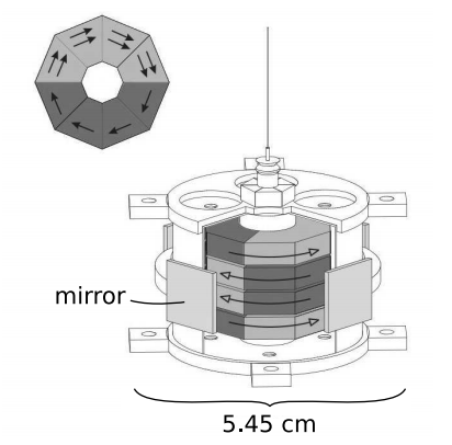
There are, however, some high-precision experiments that have a reasonable chance of detecting whether our universe has torsion. Torsion violates the equivalence principle, and by the turn of the century tests of the equivalence principle had reached a level of precision sufficient to rule out some models that include torsion. Figure 5.8.4 shows a torsion pendulum used in an experiment by the Eöt-Wash group at the University of Washington.¹¹ If torsion exists, then the intrinsic spin \(\boldsymbol{\sigma}\) of an electron should have an energy \(\boldsymbol{\sigma} \cdot \boldsymbol{\tau}\), where \(\boldsymbol{\tau}\) is the spacelike part of the torsion vector. The torsion could be generated by the earth, the sun, or some other object at a greater distance. The interaction \(\boldsymbol{\sigma} \cdot \boldsymbol{\tau}\) will modify the behavior of a torsion pendulum if the spins of the electrons in the pendulum are polarized nonrandomly, as in a magnetic material. The pendulum will tend to precess around the axis defined by \(\boldsymbol{\tau}\).

Figure \(\PageIndex{4}\) - The University of Washington torsion pendulum used to search for torsion. The light gray wedges are Alnico, the darker ones SmCo5. The arrows with the filled heads represent the directions of the electron spins, with denser arrows indicating higher polarization. The arrows with the open heads show the direction of the B field.

This type of experiment is extremely difficult, because the pendulum tends to act as an ultra-sensitive magnetic compass, resulting in a measurement of the ambient magnetic field rather than the hypothetical torsion field \(\boldsymbol{\tau}\). To eliminate this source of systematic error, the UW group first eliminated the ambient magnetic field as well as possible, using mu-metal shielding and Helmholtz coils. They also constructed the pendulum out of a combination of two magnetic materials, Alnico 5 and SmCo₅, in such a way that the magnetic dipole moment vanished, but the spin dipole moment did not; Alnico 5’s magnetic field is due almost entirely to electron spin, whereas the magnetic field of SmCo₅ contains significant contributions from orbital motion. The result was a nonmagnetic object whose spins were polarized. After four years of data collection, they found \(|\boldsymbol{\tau}| \lesssim 10^{−21}\) eV. Models that include torsion typically predict such effects to be of the order of \(\frac{m^{2}_{e}}{m_{P}} ∼ 10^{−17}\) eV, where m_e is the mass of the electron and \(m_{P} = \sqrt{\frac{\hbar c}{G}}\) ≈ 10¹⁹ GeV ≈ 20 \(\mu\)g is the Planck mass. A wide class of these models is therefore ruled out by these experiments.

Since there appears to be no experimental evidence for the existence of gravitational torsion in our universe, we will assume from now on that it vanishes identically. Einstein made the same assumption when he originally created general relativity, although he and Cartan later tinkered with non-torsion-free theories in a failed attempt to unify gravity with electromagnetism. Some models that include torsion remain viable. For example, it has been argued that the torsion tensor should fall off quickly with distance from the source.¹²

References

¹¹ http://arxiv.org/abs/hep-ph/0606218

¹² Carroll and Field, http://arxiv.org/abs/gr-qc/9403058