2.2: Flatness

Learning Objectives

• Study the concept of parallel transport
• Flatness of spacetime

Failure of Parallelism

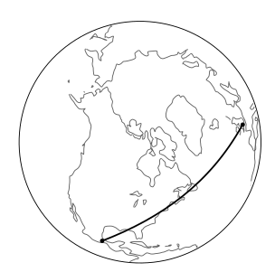
In Postulate P1 we implicitly assumed that given two points, there was a certain vector connecting them. This is analogous to the Euclidean postulate that two points define a line. For insight, let’s think about how the Euclidean version of this assumption could fail. Euclidean geometry is only an approximate description of the earth’s surface, for example, and this is why flat maps always entail distortions of the actual shapes. The distortions might be negligible on a map of Connecticut, but severe for a map of the whole world. That is, the globe is only locally Euclidean. On a spherical surface, the appropriate object to play the role of a “line” is a great circle, Figure \(\PageIndex{1}\). The lines of longitude are examples of great circles, and since these all coincide at the poles, we can see that two points do not determine a line in noneuclidean geometry.

Figure \(\PageIndex{1}\): An airplane flying from Mexico City to London follows the shortest path, which is a segment of a great circle. A path of extremal length between two points is called a geodesic.

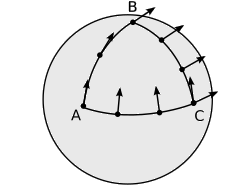
A two-dimensional bug living on the surface of a sphere would not be able to tell that the sphere was embedded in a third dimension, but it could still detect the curvature of the surface. It could tell that Euclid’s postulates were false on large distance scales. A method that has a better analog in spacetime is shown in figure \(\PageIndex{2}\): transporting a vector from one point to another depends on the path along which it was transported. This effect is our definition of curvature.

Figure \(\PageIndex{2}\): Transporting the vector along path \(\overrightarrow{AC}\) gives a different result than doing it along the path ABC.

Parallel Transport

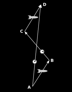
The particular type of transport that we have in mind here is called parallel transport. When I walk from the living room to the kitchen while carrying a mechanical gyroscope, I’m parallel transporting the spacelike vector indicated by the direction of its axis. Figure \(\PageIndex{3}\) shows that parallel transport can also be defined for timelike vectors, and that parallel transport can be defined in spacetime using only inertial motion, clocks, and intersection of world-lines. Observers aboard the two spaceships use clocks in order to verify the parallelism of their world-lines (vectors \(\overrightarrow{AB}\) and \(\overrightarrow{CD}\), which have equal lengths as measured by the proper time elapsed aboard the ships). Observer \(\overrightarrow{AB}\) shoots clocks to observer \(\overrightarrow{CD}\), and the clocks are set up so that when they pass by one another, they automatically record one another’s readings. The vectors are parallel if the record later reveals \(\overrightarrow{AD}\) and \(\overrightarrow{BC}\) intersected at their midpoints, as measured by the proper times recorded on the clocks.

Figure \(\PageIndex{3}\): Parallel Transport.

Special Relativity Requires Flat Spacetime

Hidden in a number of spots in Chapter 1 was the following assumption.

Postulate 2 (P2): Flatness of spacetime

Parallel-transporting a vector from one point to another gives a result that is independent of the path along which it was transported.

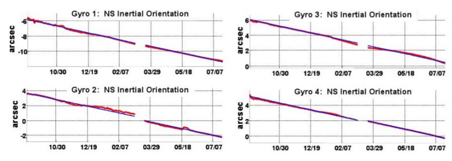
Property P2 is only approximately true, as shown explicitly by the Gravity Probe B satellite, launched in 2004. The probe carried four gyroscopes made of quartz, which were the most perfect spheres ever manufactured, varying from sphericity by no more than about \(40\) atoms. After one year and about \(5000\) orbits around the earth, the gyroscopes were found to have changed their orientations relative to the distant stars by about \(3 \times 10^{-6}\) radians (figure \(\PageIndex{4}\)). This is a violation of P2, but one that was very small and difficult to detect. The result was in good agreement with the predictions of general relativity, which describes gravity as a curvature of spacetime. The smallness of the effect tells us that the earth’s gravitational field is not so large as to completely invalidate special relativity as a description of the nearby region of spacetime.

One of the basic assumptions of general relativity is that in a small enough region of spacetime, it is always a good approximation to assume P2, so that general relativity is locally the same as special relativity. In the Gravity Probe B experiment, the effect was small and hard to detect, and this was the reason for letting the effect accumulate over a large number of orbits, spanning a large region of spacetime. Problem Q5 in the exercises section investigates more quantitatively how the size of curvature effects varies with the size of the region.

Figure \(\PageIndex{4}\): Precession angle as a function of time as measured by the four gyroscopes aboard Gravity Probe B.