1.7: Exercise problems

Exercise \(\PageIndex{1}\)

Two bodies, with temperature-independent heat capacities \(C_1\) and \(C_2\), and different initial temperatures \(T_1\) and \(T_2\), are placed into a weak thermal contact. Calculate the change of the total entropy of the system before it reaches the thermal equilibrium.

Exercise \(\PageIndex{2}\)

A gas portion has the following properties:

(i) its heat capacity \(C_V = aT^b\), and

(ii) the work \(\mathscr{W}_T\) needed for its isothermal compression from \(V_2\) to \(V_1\) equals \(cT \ln (V_2/V_1)\),

where \(a\), \(b\), and \(c\) are some constants. Find the equation of state of the gas, and calculate the temperature dependence of its entropy \(S\) and thermodynamic potentials \(E\), \(H\), \(F\), \(G\), and \(\Omega\).

Exercise \(\PageIndex{3}\)

A closed volume with an ideal classical gas of similar molecules is separated with a partition in such a way that the number \(N\) of molecules in each part is the same, but their volumes are different. The gas is initially in thermal equilibrium, and its pressure in one part is \(P_1\), and in the other part, \(P_2\). Calculate the change of entropy resulting from a fast removal of the partition, and analyze the result.

Exercise \(\PageIndex{4}\)

An ideal classical gas of \(N\) particles is initially confined to volume \(V\), and is in thermal equilibrium with a heat bath of temperature \(T\). Then the gas is allowed to expand to volume \(V’ > V\) in one the following ways:

(i) The expansion is slow, so that due to the sustained thermal contact with the heat bath, the gas temperature remains equal to \(T\).

(ii) The partition separating the volumes \(V\) and \((V’ –V)\) is removed very fast, allowing the gas to expand rapidly.

For each process, calculate the eventual changes of pressure, temperature, energy, and entropy of the gas at its expansion.

Exercise \(\PageIndex{5}\)

For an ideal classical gas with temperature-independent specific heat, derive the relation between \(P\) and \(V\) at an adiabatic expansion/compression.

Exercise \(\PageIndex{6}\)

Calculate the speed and the wave impedance of acoustic waves propagating in an ideal classical gas with temperature-independent specific heat, in the limits when the propagation may be treated as:

(i) an isothermal process, and

(ii) an adiabatic process.

Which of these limits is achieved at higher wave frequencies?

Exercise \(\PageIndex{7}\)

As will be discussed in Sec. 3.5, the so-called “hardball” models of classical particle interaction yield the following equation of state of a gas of such particles:

\[P = T \phi (n), \nonumber\]

where \(n = N/V\) is the particle density, and the function \(\phi (n)\) is generally different from that \(( \phi_{ideal}(n) = n)\) of the ideal gas, but still independent of temperature. For such a gas, with temperature-independent \(c_V\), calculate:

(i) the energy of the gas, and

(ii) its pressure as a function of \(n\) at the adiabatic compression.

Exercise \(\PageIndex{8}\)

For an arbitrary thermodynamic system with a fixed number of particles, prove the following four Maxwell relations (already mentioned in Sec. 4):

(i): \[\left(\frac{\partial S}{\partial V}\right)_{T} = \left(\frac{\partial P}{\partial T}\right)_{V},\nonumber\]	(ii): \[\left(\frac{\partial V}{\partial S}\right)_{P} = \left(\frac{\partial T}{\partial P}\right)_{S},\nonumber\]
(iii): \[\left(\frac{\partial S}{\partial P}\right)_{T} = -\left(\frac{\partial V}{\partial T}\right)_{P},\nonumber\]	(iv): \[\left(\frac{\partial P}{\partial S}\right)_{V} = -\left(\frac{\partial T}{\partial V}\right)_{S},\nonumber\]

and also the following relation:

\[\left(\frac{\partial E}{\partial V}\right)_{T} = T\left(\frac{\partial P}{\partial T}\right)_{V} - P.\nonumber\]

Exercise \(\PageIndex{9}\)

Express the heat capacity difference, \(C_P – C_V\), via the equation of state \(P = P(V, T)\) of the system.

Exercise \(\PageIndex{10}\)

\[\kappa_T \equiv - \frac{1}{V} \left(\frac{\partial V}{\partial P}\right)_{T,N}\nonumber\]

in a single-phase system may be expressed in two different ways:

\[\kappa_T = - \frac{V^2}{N^2} \left(\frac{\partial^2 P}{\partial \mu^2}\right)_{T} = \frac{V}{N^2} \left(\frac{\partial N}{\partial \mu}\right)_{T,V}. \nonumber\]

Exercise \(\PageIndex{11}\)

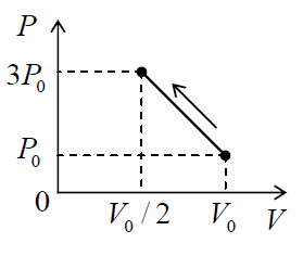
A reversible process, performed with a fixed portion of an ideal classical gas, may be represented on the \([V, P]\) plane with the straight line shown in the figure on the right. Find the point at which the heat flow into/out of the gas changes its direction.

Exercise \(\PageIndex{12}\)

Two bodies have equal, temperature-independent heat capacities \(C\), but different temperatures, \(T_1\) and \(T_2\). Calculate the maximum mechanical work obtainable from this system, using a heat engine.

Exercise \(\PageIndex{13}\)

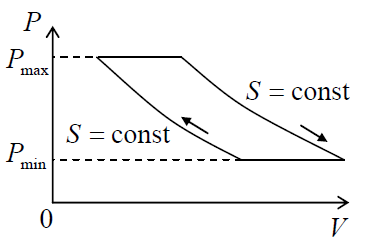
Express the efficiency \(\eta\) of a heat engine that uses the so called Joule cycle, consisting of two adiabatic and two isobaric processes (see the figure on the right), via the minimum and maximum values of pressure, and compare the result with \(\eta_{Carnot}\). Assume an ideal classical working gas with temperature-independent \(C_P\) and \(C_V\).

Exercise \(\PageIndex{14}\)

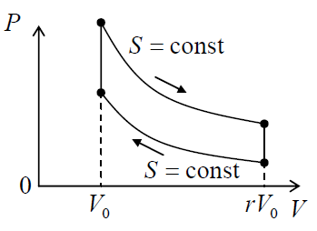
Calculate the efficiency of a heat engine using the Otto cycle,⁴⁷ which consists of two adiabatic and two isochoric (constant volume) reversible processes – see the figure on the right. Explore how the efficiency depends on the ratio \(r \equiv V_{max}/V_{min}\), and compare it with the Carnot cycle’s efficiency. Assume an ideal classical working gas with temperature-independent heat capacity.

Exercise \(\PageIndex{15}\)

A heat engine’s cycle consists of two isothermal (\(T =\) const) and two isochoric (\(V =\) const) reversible processes – see the figure on the right.⁴⁸

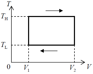
(i) Assuming that the working gas is an ideal classical gas of \(N\) particles, calculate the mechanical work performed by the engine during one cycle.

(ii) Are the specified conditions sufficient to calculate the engine’s efficiency? (Justify your answer.)

Exercise \(\PageIndex{16}\)

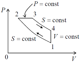
The Diesel cycle (an approximate model of the Diesel internal combustion engine’s operation) consists of two adiabatic processes, one isochoric process, and one isobaric process – see the figure on the right. Assuming an ideal working gas with temperature independent \(C_V\) and \(C_P\), express the efficiency \(\eta\) of the heat engine using this cycle via the gas temperature values in its transitional states corresponding to the corners of the cycle diagram.

---

Footnotes

1. For remedial reading, I can recommend, for example (in the alphabetical order): C. Kittel and H. Kroemer, Thermal Physics, \(2^{nd}\) ed., W. H. Freeman (1980); F. Reif, Fundamentals of Statistical and Thermal Physics, Waveland (2008); D. V. Schroeder, Introduction to Thermal Physics, Addison Wesley (1999).
2. Here “internal” is an (admittedly loose) term meaning all the physics unrelated to the motion of the system as a whole. The most important example of internal dynamics is the thermal motion of atoms and molecules.
3. This is perhaps my best chance for a reverent mention of Democritus (circa 460-370 BC) – the Ancient Greek genius who was apparently the first one to conjecture the atomic structure of matter.
4. See, e.g., CM Chapters 8 and 9.
5. In order to prove that, it is sufficient to integrate the scalar product \(d\mathscr{W} = d\pmb{\mathscr{F}} \cdot d\mathbf{r}\), with \(d\pmb{\mathscr{F}} = –\mathbf{n}Pd^2r\), where \(d\mathbf{r}\) is the surface displacement vector (see, e.g., CM Sec. 7.1), and \(\mathbf{n}\) is the outer normal, over the surface.
6. See, e.g., CM Chapters 2 and 10.
7. Some of my students needed an effort to reconcile the positive signs in Eqs. (\(1.1.2-1.1.3\)) with the negative sign in the well-known relation \(dU_k = –\pmb{\mathscr{E}}(\mathbf{r}_k)d \pmb{\mathcal{p}}_k\) for the potential energy of a dipole in an external electric field – see, e.g., EM Eqs. (3.15). The resolution of this paradox is simple: each term of Equation (\(1.1.3\)) describes the work \(d\mathscr{W}_k\) of the electric field on the internal degrees of freedom of the \(k^{th}\) dipole, changing its internal energy \(E_k: dE_k = d\mathscr{W}_k\). This energy change may be viewed as coming from the dipole’s potential energy in the field: \(dE_k = –dU_k\).
8. Here, as in all my series, I am using the SI units; for their translation to the Gaussian units, I have to refer the reader to the EM part of the series.
9. Note that in systems of discrete particles, most generalized forces, including the fields \(\pmb{\mathscr{E}}\) and \(\pmb{\mathscr{H}}\), differ from the pressure \(P\) in the sense that their work may be explicitly partitioned into single-particle components – see Eqs. (\(1.1.3\)) and (\(1.1.5\)). This fact gives some discretion for the calculations based on thermodynamic potentials – see Sec.4.
10. The notion of entropy was introduced into thermodynamics in 1865 by Rudolf Julius Emanuel Clausius on a purely phenomenological basis. In the absence of a clue about the entropy’s microscopic origin (which had to wait for the works by L. Boltzmann and J. Maxwell), this was an amazing intellectual achievement.
11. Because of that, the possibility of the irreversible macroscopic behavior of microscopically reversible systems was questioned by some serious scientists as recently as in the late \(19^{th}\) century – notably by J. Loschmidt in 1876.
12. While quantum-mechanical effects, with their intrinsic uncertainty, may be quantitatively important in this example, our qualitative discussion does not depend on them. Another classical example is the chaotic motion of a ball on a 2D Sinai billiard – see CM Chapter 9 and in particular Figure 9.8 and its discussion.
13. Several other quantities, for example the heat capacity \(C\), may be calculated as partial derivatives of the basic variables discussed above. Also, at certain conditions, the number of particles \(N\) in a certain system may be not fixed and also considered as an (extensive) variable – see Sec. 5 below.
14. Admittedly, some of these proofs are based on other plausible but deeper postulates, for example the central statistical hypothesis (Sec. 2.2), whose best proof, to my knowledge, is just the whole body of experimental data.
15. Implicitly, this statement also postulates the existence, in a closed system, of thermodynamic equilibrium, an asymptotically reached state in which all macroscopic variables, including entropy, remain constant. Sometimes this postulate is called the \(0^{th}\) law of thermodynamics.
16. Two initial formulations of this law, later proved equivalent, were put forward independently by Lord Kelvin (born William Thomson) in 1851 and by Rudolf Clausius in 1854.
17. Here we strongly depend on a very important (and possibly the least intuitive) aspect of the \(2^{nd}\) law, namely that the entropy is a unique measure of disorder.
18. Here I have to mention a traditional unit of thermal energy, the calorie, still being used in some applied fields. In the most common modern definition (as the so-called thermochemical calorie) it equals exactly 4.148 J.
19. For the more exact values of this and other constants, see appendix CA: Selected Physical Constants. Note that both \(T\) and \(T_K\) define the natural absolute (also called “thermodynamic”) scale of temperature, vanishing at the same point – in contrast to such artificial scales as the degrees Celsius (“centigrades”), defined as \(T_C \equiv T_K + 273.15\), or the degrees Fahrenheit: \(T_F \equiv (9/5)T_C + 32\).
20. Historically, such notion was initially qualitative – just as something distinguishing “hot” from “cold”. After the invention of thermometers (the first one by Galileo Galilei in 1592), mostly based on thermal expansion of fluids, this notion had become quantitative but not very deep: being understood as something “what the thermometer measures” – until its physical sense as a measure of thermal motion’s intensity, was revealed in the \(19^{th}\) century.
21. Let me emphasize again that any adiabatic process is reversible, but not vice versa.
22. Such conservation, expressed by Eqs. (\(1.3.5\))-(\(1.3.6\)), is commonly called the \(1^{st}\) law of thermodynamics. While it (in contrast with the \(2^{nd}\) law) does not present any new law of nature, and in particular was already used de-facto to write the first of Eqs. (\(1.2.2\)) and also Equation (\(1.3.1\)), such a grand name was absolutely justified in the \(19^{th}\) century when the mechanical nature of the internal energy (the thermal motion) was not at all clear. In this context, the names of three scientists, Benjamin Thompson (who gave, in 1799, convincing arguments that heat cannot be anything but a form of particle motion), Julius Robert von Mayer (who conjectured the conservation of the sum of the thermal and macroscopic mechanical energies in 1841), and James Prescott Joule (who proved this conservation experimentally two years later), have to be reverently mentioned.
23. Actually, the \(3^{rd}\) law (also called the Nernst theorem) as postulated by Walter Hermann Nernst in 1912 was different – and really meaningful: “It is impossible for any procedure to lead to the isotherm \(T = 0\) in a finite number of steps.” I will discuss this theorem at the end of Sec. 6.
24. By this definition, the full heat capacity of a system is an extensive variable, but it may be used to form such intensive variables as the heat capacity per particle, called the specific heat capacity, or just the specific heat. (Please note that the last terms are rather ambiguous: they are used for the heat capacity per unit mass, per unit volume, and sometimes even for the heat capacity of the system as the whole, so that some caution is in order.)
25. Dividing both sides of Equation (\(1.3.6\)) by \(dT\), we get the general relation \(dQ/dT = TdS/dT\), which may be used to rewrite the definitions (\(1.3.9\)) and (\(1.3.10\)) in the following forms: \[C_V = T \left( \frac{\partial S}{\partial T} \right)_V, \quad C_P = T \left( \frac{\partial S}{\partial T} \right)_P, \nonumber\] more convenient for some applications.
26. From the point of view of mathematics, Equation (\(1.4.4\)) is a particular case of the so-called Legendre transformations.
27. This function (as well as the Gibbs free energy \(G\), see below), had been introduced in 1875 by J. Gibbs, though the term “enthalpy” was coined (much later) by H. Onnes.
28. It was named after Hermann von Helmholtz (1821-1894). The last of the listed terms for \(F\) was recommended by the most recent (1988) IUPAC’s decision, but I will use the first term, which prevails is physics literature. The origin of the adjective “free” stems from Equation (\(1.4.9\)): \(F\) is may be interpreted as the internal energy’s part that is “free” to be transferred to the mechanical work, at the (most common) reversible, isothermal process.
29. Note the similarity of this situation with that is analytical mechanics (see, e.g., CM Chapters 2 and 10): the Lagrangian function may be used to derive the equations of motion if it is expressed as a function of generalized coordinates and their velocities, while to use the Hamiltonian function in a similar way, it has to be expressed as a function of the generalized coordinates and the corresponding momenta.
30. There is also a wealth of other relations between thermodynamic variables that may be represented as second derivatives of the thermodynamic potentials, including four Maxwell relations such as \((\partial S/\partial V)_T = (\partial P/\partial T)_V\), etc. (They may be readily recovered from the well-known property of a function of two independent arguments, say, \(f(x, y): \partial (\partial f/\partial x)/\partial y = \partial (\partial f/\partial y)/\partial x.)\) In this chapter, I will list only the thermodynamic relations that will be used later in the course; a more complete list may be found, e.g., in Sec. 16 of the book by L. Landau and E. Lifshitz, Statistical Physics, Part 1, \(3^{rd}\) ed., Pergamon, 1980 (and its later re-printings).
31. There are a few practicable systems, notably including the so-called adiabatic magnetic refrigerators (to be discussed in Chapter 2), where the unintentional growth of \(S\) is so slow that the condition \(S =\) const may be closely approached.
32. It is convenient to describe it as the difference between the “usual” (internal) potential energy \(U\) of the system to its “Gibbs potential energy” \(U_G\) – see CM Sec. 1.4. For the readers who skipped that discussion: my pet example is the usual elastic spring with \(U = kx^{2}/2\), under the effect of an external force \(\mathscr{F}\), whose equilibrium position \((x_0 = \mathscr{F}/k)\) evidently corresponds to the minimum of \(U_G = U – \mathscr{F}_x\), rather than just \(U\).
33. An example of such an extreme situation is the case when an external magnetic field \(\pmb{\mathscr{H}}\) is applied to a superconductor in its so-called intermediate state, in which the sample partitions into domains of the “normal” phase with \(\pmb{\mathscr{B}} = \mu_0\pmb{\mathscr{H}}\), and the superconducting phase with \(\pmb{\mathscr{B}} = 0\). In this case, the field is effectively applied to the interfaces between the domains, very similarly to the mechanical pressure applied to a gas portion via a piston – see Figure \(1.1.1\) again.
34. The long history of the gradual discovery of this relation includes the very early (circa 1662) work by R. Boyle and R. Townely, followed by contributions from H. Power, E. Mariotte, J. Charles, J. Dalton, and J. Gay-Lussac. It was fully formulated by Benoît Paul Émile Clapeyron in 1834, in the form \(PV = nRT_K\), where \(n\) is the number of moles in the gas sample, and \(R \approx 8.31\) J/mole \(\cdot\) K is the so-called gas constant. This form is equivalent to Equation (\(1.4.21\)), taking into account that \(R \equiv k_BN_A\), where \(N_A = 6.022\) \(140\) \(76 \times 10^{23}\) mole\(^{-1}\) is the Avogadro number, i.e. the number of molecules per mole. (By the mole’s definition, \(N_A\) is just the reciprocal mass, in grams, of the \(1/12^{th}\) part of the \(^{12}\)C atom, which is close to the mass of one proton or neutron – see Appendix CA: Selected Physical Constants.) Historically, this equation of state was the main argument for the introduction of the absolute temperature \(T\), because only with it, the equation acquires the spectacularly simple form (\(1.4.21\)).
35. Note that Equation (\(1.4.24\)), in particular, describes a very important property of the ideal classical gas: its energy depends only on temperature (and the number of particles), but not on volume or pressure.
36. Note, however, that the difference \(C_P – C_V = N\) is independent of \(f(T)\). (If the temperature is measured in kelvins, this relation takes a more familiar form \(C_P – C_V = nR\).) It is straightforward (and hence left for the reader’s exercise) to show that the difference \(C_P – C_V\) of any system is fully determined by its equation of state.
37. Another important example is a gas in a contact with the open-surface liquid of similar molecules.
38. This name, of a historic origin, is misleading: as evident from Equation (\(1.5.1\)), \(\mu\) has a clear physical sense of the average energy cost of adding one more particle to the system of \(N >> 1\) particles.
39. Note that strictly speaking, Eqs. (\(1.2.6\)), (\(1.3.2\)), (\(1.4.8\)), (\(1.4.12\)). and (\(1.4.16\)) should be now generalized by adding another lower index, \(N\), to the corresponding derivatives; I will just imply this.
40. The whole field of thermodynamics was spurred by the famous 1824 work by Nicolas Léonard Sadi Carnot, in which he, in particular, gave an alternative, indirect form of the \(2^{nd}\) law of thermodynamics – see below.
41. Curiously, S. Carnot derived his key result still believing that heat is some specific fluid (“caloric”), whose flow is driven by the temperature difference, rather than just a form of particle motion.
42. Semi-quantitatively, such trend is valid also for other, less efficient but more practicable heat engine cycles – see Problems 13-16. This trend is the leading reason why internal combustion engines, with \(T_H\) of the order of 1,500 K, are more efficient than steam engines, with the difference \(T_H – T_L\) of at most a few hundred K.
43. In some alternative axiomatic systems of thermodynamics, this fact is postulated and serves the role of the \(2^{nd}\) law. This is why it is under persisting (dominantly, theoretical) attacks by suggestions of more efficient heat engines – recently, mostly of quantum systems using sophisticated protocols such as the so-called shortcut-to adiabaticity – see, e.g., the recent paper by O. Abah and E. Lutz, Europhysics Lett. 118, 40005 (2017), and references therein. To the best of my knowledge, reliable analyses of all the suggestions put forward so far have confirmed that the Carnot efficiency (\(1.6.6\)) is the highest possible even in quantum systems.
44. Such a hypothetical heat engine, which would violate the \(2^{nd}\) law of thermodynamics, is called the “perpetual motion machine of the \(2^{nd}\) kind” – in contrast to any (also hypothetical) “perpetual motion machine of the \(1^{st}\) kind” that would violate the \(1^{st}\) law, i.e., the energy conservation.
45. Note that for such metastable systems as glasses the situation may be more complicated. (For a detailed discussion of this issue see, e.g., J. Wilks, The Third Law of Thermodynamics, Oxford U. Press, 1961.) Fortunately, this issue does not affect other aspects of statistical physics – at least those to be discussed in this course.
46. Note that the compressibility is just the reciprocal bulk modulus, \(\kappa = 1/K\) – see, e.g., CM Sec. 7.3.
47. This name stems from the fact that the cycle is an approximate model of operation of the four-stroke internal combustion engine, which was improved and made practicable (though not invented!) by N. Otto in 1876.
48. The reversed cycle of this type is a reasonable approximation for the operation of the Stirling and Gifford McMahon (GM) refrigerators, broadly used for cryocooling – for a recent review see, e.g., A. de Waele, J. Low Temp. Phys. 164, 179 (2011).