3.4: The Bose-Einstein condensation

BEC: critical temperature

\[\boxed{T_c = T_0 \left[ \frac{1}{\sqrt{2}\pi^2} \int^{\infty}_0 \frac{\xi^{1/2}d\xi}{e^{\xi}-1}\right]^{-2/3} = T_0 \left[ \frac{1}{\sqrt{2}\pi^2} \Gamma \left(\frac{3}{2}\right) \zeta \left(\frac{3}{2}\right)\right]^{-2/3} \approx 3.313 T_0,} \label{71}\]

the result explaining the \(T_c/T_0\) ratio mentioned in Sec. 2 and indicated in Figure \(3.2.1\).

Figure \(\PageIndex{1}\): The Bose-Einstein condensation: (a) the chemical potential of the gas and (b) its pressure, as functions of temperature. The dashed line corresponds to the classical gas.

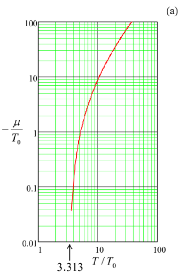
Let us have a good look at the temperature interval \(0 < T < T_c\), which cannot be directly described by Equation (\(3.2.11\)) (with the appropriate negative sign in the denominator), and hence may look rather mysterious. Indeed, within this range, the chemical potential \(\mu \), cannot either be negative or equal zero, because according to Equation (\ref{71}), in this case, Equation (\(3.2.11\)) would give a value of \(N\) smaller than the number of particles we actually have. On the other hand, \(\mu\) cannot be positive either, because the integral (\(3.2.11\)) would diverge at \(\varepsilon \rightarrow \mu\) due to the divergence of \(\langle N(\varepsilon )\rangle\) – see, e.g., Figure \(2.8.2\). The only possible resolution of the paradox, suggested by A. Einstein in 1925, is as follows: at \(T < T_c\), the chemical potential of each particle of the system still equals exactly zero, but a certain number (\(N_0\) of \(N\)) of them are in the ground state (with \(\varepsilon \equiv p^2/2m = 0\)), forming the so-called Bose-Einstein condensate, usually referred to as the BEC. Since the condensate particles do not contribute to Equation (\(3.2.11\)) (because of the factor \(\varepsilon^{1/2} = 0\)), their number \(N_0\) may be calculated by using that formula (or, equivalently, Equation (\(3.2.15\))), with \(\mu = 0\), to find the number (\(N – N_0\)) of particles still remaining in the gas, i.e. having energy \(\varepsilon > 0\):

\[N-N_0 = \frac{gV(mT)^{3/2}}{\sqrt{2}\pi^2\hbar^3}\int^{\infty}_0\frac{\xi^{1/2}d\xi}{e^{\xi}-1}.\label{72}\]

\[N=\frac{gV(mT_c)^{3/2}}{\sqrt{2}\pi^2\hbar^3}\int^{\infty}_0\frac{\xi^{1/2}d\xi}{e^{\xi}-1}.\label{73}\]

Dividing both sides of Eqs. (\ref{72}) and (\ref{73}), we get an extremely simple and elegant result:

\[\frac{N-N_0}{N} = \left(\frac{T}{T_c}\right)^{3/2}, \quad \text{ so that } N_0 = N\left[1-\left(\frac{T}{T_c}\right)^{3/2}\right], \text{ for }T\leq T_c. \label{74a}\]

Please note that this result is only valid for the particles whose motion, within the volume \(V\), is free – in other words, for a system of free particles confined within a rigid-wall box of volume \(V\). In most experiments with the Bose-Einstein condensation of dilute gases of neutral (and hence very weakly interacting) atoms, they are held not in such a box, but at the bottom of a “soft” potential well, which may be well approximated by a 3D quadratic parabola: \(U(\mathbf{r}) = m\omega^2r^2/2\). It is straightforward (and hence left for the reader’s exercise) to show that in this case, the dependence of \(N_0(T)\) is somewhat different:

\[N_0 = N\left[1-\left(\frac{T}{T^*_c}\right)^{3}\right], \text{ for } T \leq T^*_c, \label{74b}\]

where \(T_c^*\) is a different critical temperature, which now depends on \(\hbar \omega \), i.e. on the confining potential’s “steepness”. (In this case, \(V\) is not exactly fixed; however, the effective volume occupied by the particles at \(T = T_c^*\) is related to this temperature by a formula close to Equation (\ref{71}), so that all estimates given above are still valid.) Figure \(\PageIndex{2}\) shows one of the first sets of experimental data for the Bose-Einstein condensation of a dilute gas of neutral atoms. Taking into account the finite number of particles in the experiment, the agreement with the simple theory is surprisingly good.

\[E(T_c) = gV \frac{m^{3/2}T_c^{5/2}}{\sqrt{2}\pi^2\hbar^3} \int^{\infty}_0 \frac{\xi^{3/2} d\xi}{e^{\xi}-1} = gV \frac{m^{3/2}T_c^{5/2}}{\sqrt{2}\pi^2\hbar^3} \Gamma \left(\frac{5}{2}\right) \zeta \left(\frac{5}{2}\right) \approx 0.7701 \ NT_c, \label{75}\]

so that using the universal relation (\(3.2.19\)), we get the pressure value,

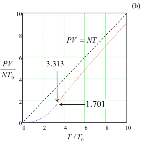
\[P(T_c) = \frac{2}{3} \frac{E(T_c)}{V} = \frac{\zeta (5/2)}{\zeta (3/2)} \frac{ N}{V} T_c \approx 0.5134 \frac{N}{V} T_c \approx 1.701 \ P_0, \label{76}\]

which is somewhat lower than, but comparable to \(P(0)\) for the fermions – cf. Equation (\(3.3.6\)).

Figure \(\PageIndex{2}\): The total number \(N\) of trapped \(^{87}\)Rb atoms (inset) and their ground-state fraction \(N_0/N\), as functions of the ratio \(T/T_c\), as measured in one of the pioneering experiments – see J. Ensher et al., Phys. Rev. Lett. 77, 4984 (1996). In this experiment, \(T_c^*\) was as low as \(0.28 \times 10^{-6}\) K. The solid line shows the simple theoretical dependence \(N(T)\) given by Equation (\ref{74b}), while other lines correspond to more detailed theories taking into account the finite number \(N\) of trapped atoms. atoms. © 1996 APS, reproduced with permission.

Now we can use the same Equation (\(3.2.23\)), also with \(\mu = 0\), to calculate the energy of the gas at \(T<T_c\),

\[E(T) = gV \frac{m^{3/2}T^{5/2}}{\sqrt{2}\pi^2\hbar^3} \int^{\infty}_0 \frac{\xi^{3/2} d\xi}{e^{\xi}-1}.\label{77}\]

Comparing this relation with the first form of Equation (\ref{75}), which features the same integral, we immediately get one more simple temperature dependence:

BEC: energy

\[\boxed{E(T) = E(T_c) \left(\frac{T}{T_c}\right)^{5/2}, \text{ for } T \leq T_c. }\label{78}\]

From the universal relation (\(3.2.19\)), we immediately see that the gas pressure follows the same dependence:

BEC: pressure

\[\boxed{P(T) = P(T_c) \left(\frac{T}{T_c}\right)^{5/2}, \text{ for } T \leq T_c. }\label{79}\]

This temperature dependence of pressure is shown with the blue line in Figure \(\PageIndex{1b}\). The plot shows that for all temperatures (both below and above \(T_c\)) the pressure is lower than that of the classical gas of the same density. Now note also that since, according to Eqs. (\(3.3.6\)) and (\ref{76}), \(P(T_c) \propto P_0 \propto V^{-5/3}\), while according to Eqs. (\(3.2.6\)) and (\ref{71}), \(T_c \propto T_0 \propto V^{-2/3}\), the pressure (\ref{79}) is proportional to \(V^{-5/3}/(V^{-2/3})^{5/2} = V^0\), i.e. does not depend on the volume at all! The physics of this result (which is valid at \(T < T_c\) only) is that as we decrease the volume at a fixed total number \(N\) of particles, more and more of them go to the condensate, decreasing the number (\(N – N_0\)) of particles in the gas phase, but not changing its spatial density pressure. Such behavior is very typical for the coexistence of two different phases of the same matter – see, in particular, the next chapter.

The last thermodynamic variable of major interest is heat capacity, because it may be most readily measured. For temperatures \(T \leq T_c\), it may be easily calculated from Equation (\ref{78}):

\[C_V (T) \equiv \left( \frac{\partial E}{\partial T} \right)_{N,V} = E(T_c) \frac{5}{2} \frac{T^{3/2}}{T_c^{5/2}}, \label{80}\]

so that below \(T_c\), the capacity increases with temperature, at the critical temperature reaching the value

\[C_V (T_c) = \frac{5}{2} \frac{E(T_c)}{T_c} \approx 1.925 \ N, \label{81}\]

which is approximately 28% above that (\(3N/2\)) of the classical gas. (As a reminder, in both cases we ignore possible contributions from the internal degrees of freedom.) The analysis for \(T \geq T_c\) is a little bit more cumbersome because differentiating \(E\) over temperature – say, using Equation (\(3.2.23\)) – one should also take into account the temperature dependence of \(\mu\) that follows from Equation (\(3.2.11\)) – see also Figure \(\PageIndex{1}\). However, the most important feature of the result may be predicted without the calculation (which is being left for the reader’s exercise). Namely, since at \(T >> T_c\) the heat capacity has to approach the classical value \(1.5N\), starting from the value (\ref{81}), it must decrease with temperature at \(T > T_c\), thus forming a sharp maximum (a “cusp”) at the critical point \(T = T_c\) – see Figure \(\PageIndex{3}\).

Figure \(\PageIndex{3}\): Temperature dependences of the heat capacity of an ideal Bose-Einstein gas, numerically calculated from Eqs. (\(3.2.23\)) and (\(3.2.11\)) for \(T \geq T_c\), and given by Equation (\ref{80}) for \(T \leq T_c\).

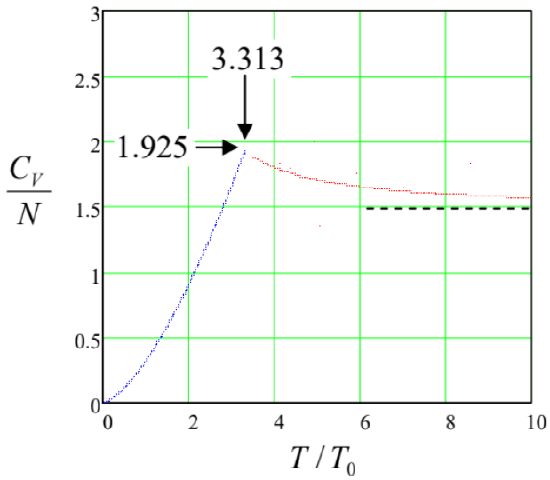
Such a cusp is a good indication of the Bose-Einstein condensation in virtually any experimental system, especially because inter-particle interactions (unaccounted for in our simple discussion) typically make this feature even more substantial, frequently turning it into a weak (logarithmic) singularity. Historically, such a singularity was the first noticed, though not immediately understood sign of the Bose-Einstein condensation, observed in 1931 by W. Keesom and K. Clusius in liquid ⁴He at its \(\lambda \)-point (called so exactly because of the characteristic shape of the \(C_V(T)\) dependence) \(T = T_c \approx 2.17\) K. Other milestones of the Bose-Einstein condensation studies include:

• the experimental discovery of superconductivity (which was later explained as the result of the Bose-Einstein condensation of electron pairs) by H. Kamerlingh-Onnes in 1911;
• the development of the Bose-Einstein statistics, and predicting the condensation, by S. Bose and A. Einstein, in 1924-1925;
• the discovery of superfluidity in liquid \(^4\)He by P. Kapitza and (independently) by J. Allen and D. Misener in 1937, and its explanation as a result of the Bose-Einstein condensation by F. and H. Londons and L. Titza, with further significant elaborations by L. Landau – all in 1938;
• the explanation of superconductivity as a result of electron binding into Cooper pairs, with a simultaneous Bose-Einstein condensation of the resulting bosons, by J. Bardeen, L. Cooper, and J. Schrieffer in 1957;
• the discovery of superfluidity of two different phases of \(^3\)He, due to the similar Bose-Einstein condensation of pairs of its fermion atoms, by D. Lee, D. Osheroff, and R. Richardson in 1972;
• the first observation of the Bose-Einstein condensation in dilute gases (\(^{87}\)Ru by E. Cornell, C. Wieman, et al., and \(^{23}\)Na by W. Ketterle et al.) in 1995.

The importance of the last achievement stems from the fact that in contrast to other Bose Einstein condensates, in dilute gases (with the typical density \(n\) as low as \(\sim 10^{14}\) cm\(^{-3}\)) the particles interact very weakly, and hence many experimental results are very close to the simple theory described above and its straightforward elaborations – see, e.g., Figure \(\PageIndex{2}\).³⁵ On the other hand, the importance of other Bose-Einstein condensates, which involve more complex and challenging physics, should not be underestimated – as it sometimes is.

Perhaps the most important feature of any Bose-Einstein condensate is that all \(N_0\) condensed particles are in the same quantum state, and hence are described by exactly the same wavefunction. This wavefunction is substantially less “feeble” than that of a single particle – in the following sense. In the second quantization language,³⁶ the well-known Heisenberg’s uncertainty relation may be rewritten for the creation/annihilation operators; in particular, for bosons,

\[\left| \delta \hat{a} \delta \hat{a}^{\dagger}\right| \geq 1. \label{82}\]

Since \(\hat{a}\) and \(\hat{a}^{\dagger}\) are the quantum-mechanical operators of the complex amplitude \(a = A\text{exp}\{i\varphi \}\) and its complex conjugate \(a^* = A\text{exp}\{–i\varphi \}\), where \(A\) and \(\varphi\) are real amplitude and phase of the wavefunction, Equation (\ref{82}) yields the following approximate uncertainty relation (strict in the limit \(\delta \varphi << 1\)) between the number of particles \(N = AA^*\) and the phase \(\varphi \):

\[ \delta N\delta \varphi \geq 1/2 . \label{83}\]

This means that a condensate of \(N >> 1\) bosons may be in a state with both phase and amplitude of the wavefunction behaving virtually as \(c\)-numbers, with very small relative uncertainties: \(\delta N << N, \delta \varphi << 1\). Moreover, such states are much less susceptible to perturbations by experimental instruments. For example, the electric current carried along a superconducting wire by a coherent Bose-Einstein condensate of Cooper pairs may be as high as hundreds of amperes. As a result, the “strange” behaviors predicted by the quantum mechanics are not averaged out as in the usual particle ensembles (see, e.g., the discussion of the density matrix in Sec. 2.1), but may be directly revealed in macroscopic, measurable dynamics of the condensate.

For example, the density \(\mathbf{j}\) of the electric “supercurrent” of the Cooper pairs may be described by the same formula as the well-known usual probability current density of a single quantum particle,³⁷ just multiplied by the electric charge \(q = –2e\) of a single pair, and the pair density \(n\):

\[\mathbf{j} = qn \frac{\hbar}{m} \left( \boldsymbol{\nabla} \varphi - \frac{q}{\hbar} \mathbf{A}\right), \label{84}\]

where \(\mathbf{A}\) is the vector potential of the (electro)magnetic field. If a superconducting wire is not extremely thin, the supercurrent does not penetrate into its interior.³⁸ As a result, the integral of Equation (\ref{84}), taken along a closed superconducting loop, inside its interior (where \(\mathbf{j} = 0\)), yields

\[\frac{q}{\hbar} \oint_C \mathbf{A} \cdot d\mathbf{r} = \Delta \varphi = 2\pi M, \label{85}\]

where \(M\) is an integer. But, according to the basic electrodynamics, the integral on the left-hand side of this relation is nothing more than the flux \(\Phi\) of the magnetic field \(\pmb{\mathscr{B}}\) piercing the wire loop area \(A\). Thus we immediately arrive at the famous magnetic flux quantization effect:

\[\Phi \equiv \int_A \mathscr{B}_n d^2 r = M \Phi_0, \quad \text{ where } \Phi_0 \equiv \frac{2\pi \hbar }{|q|} \approx 2.07 \times 10^{-15} \text{Wb}, \label{86}\]

which was theoretically predicted in 1950 and experimentally observed in 1961. Amazingly, this effect holds even “over miles of dirty lead wire”, citing H. Casimir’s famous expression, sustained by the coherence of the Bose-Einstein condensate of Cooper pairs.

Other prominent examples of such macroscopic quantum effects in Bose-Einstein condensates include not only the superfluidity and superconductivity as such, but also the Josephson effect, quantized Abrikosov vortices, etc. Some of these effects are briefly discussed in other parts of this series.³⁹