3.2: Calculating Chemical Potentials

Now let us discuss properties of ideal gases of free, indistinguishable particles in more detail, paying special attention to the chemical potential $\mu$ – which, for some readers, may still be a somewhat mysterious aspect of the Fermi and Bose distributions. Note again that particle indistinguishability requires the absence of thermal excitations of their internal degrees of freedom, so that in the balance of this chapter such excitations will be ignored, and the particle’s energy $\varepsilon_k$ will be associated with its “external” energy alone: for a free particle in an ideal gas, with its kinetic energy ($3.1.3$).

Let us start from the classical gas, and recall the conclusion of thermodynamics that $\mu$ is just the Gibbs potential per unit particle – see Equation ($1.5.7$). Hence we can calculate $\mu = G/N$ from Eqs. ($1.4.26$) and ($3.1.17$). The result,

$$\mu = -T \ln \frac{V}{N} + f(T) + T \ln \left[\frac{N}{gV}\left(\frac{2\pi\hbar^2}{mT}\right)^{3/2}\right],\label{32a}$$

which may be rewritten as

$$\text{exp}\left\{\frac{\mu}{T}\right\}=\frac{N}{gV}\left(\frac{2\pi\hbar^2}{mT}\right)^{3/2},\label{32b}$$

gives us some information about $\mu$ not only for a classical gas but for quantum (Fermi and Bose) gases as well. Indeed, we already know that for indistinguishable particles, the Boltzmann distribution ($2.8.1$) is valid only if $\langle N_k \rangle << 1$. Comparing this condition with the quantum statistics ($2.8.5$) and ($2.8.8$), we see again that the condition of the gas behaving classically may be expressed as

$$\text{exp}\left\{\frac{\mu-\varepsilon_k}{T}\right\}<<1\label{33}$$

for all $\varepsilon_k$. Since the lowest value of $\varepsilon_k$ given by Equation ($3.1.3$) is zero, Equation ($\ref{33}$) may be satisfied only if $\text{exp}\{\mu /T\} << 1$. This means that the chemical potential of a classical gas has to be not just negative, but also “strongly negative” in the sense

$$-\mu>>T.\label{34a}$$

According to Equation ($\ref{32a}$-$\ref{32b}$), this important condition may be represented as

$$T>>T_0,\label{34b}$$

with $T_0$ defined as

Quantum scale of temperature:

$$\boxed{T_{0} \equiv \frac{\hbar^{2}}{m}\left(\frac{N}{g V}\right)^{2 / 3} \equiv \frac{\hbar^{2}}{m}\left(\frac{n}{g}\right)^{2 / 3} \equiv \frac{\hbar^{2}}{g^{2 / 3} m r_{\text {ave }}^{2}},}\label{35}$$

where $r_{ave}$ is the average distance between the gas particles:

$$r_{ave} \equiv \frac{1}{n^{1/3}}=\left(\frac{V}{N}\right)^{1/3}.\label{36}$$

In this form, the condition ($\ref{34a}$-$\ref{34b}$) is very transparent physically: disregarding the factor $g^{2/3}$ (which is typically of the order of 1), it means that the average thermal energy of a particle, which is always of the order of $T$, has to be much larger than the energy of quantization of particle’s motion at the length $r_{ave}$. An alternative form of the same condition is¹⁹

$$r_{\mathrm{ave}}>>g^{-1 / 3} r_{\mathrm{c}}, \quad \text { where } r_{\mathrm{c}} \equiv \frac{\hbar}{(m T)^{1 / 2}}. \label{37}$$

For a typical gas (say, $\ce{N2}$, with $m \approx 14m_p \approx 2.3 \times 10^{-26}$ kg) at the standard room temperature ($T = k_B \times 300$ K $\approx 4.1 \times 10^{-21}$ J), the correlation length $r_c$ is close to $10^{-11}$ m, i.e. is significantly smaller than the physical size $a \sim 3 \times 10^{-10}$ m of the molecule. This estimate shows that at room temperature, as soon as any practical gas is rare enough to be ideal ($r_{ave} >> a$), it is classical, i.e. the only way to observe quantum effects in the translational motion of molecules is very deep refrigeration. According to Equation ($\ref{37}$), for the same nitrogen molecule, taking $r_{ave} \sim 10^2a \sim 10^{-8}$ m (to ensure that direct interaction effects are negligible), the temperature should be well below 1 mK.

In order to analyze quantitatively what happens with gases when $T$ is reduced to such low values, we need to calculate $\mu$ for an arbitrary ideal gas of indistinguishable particles. Let us use the lucky fact that the Fermi-Dirac and the Bose-Einstein statistics may be represented with one formula:

$$\langle N(\varepsilon)\rangle = \frac{1}{e^{(\varepsilon-\mu)/T}\pm 1},\label{38}$$

where (and everywhere in the balance of this section) the top sign stands for fermions and the lower one for bosons, to discuss fermionic and bosonic ideal gases in one shot.

If we deal with a member of the grand canonical ensemble (Figure $2.7.1$), in which not only $T$ but also $\mu$ is externally fixed, we may use Equation ($\ref{38}$) to calculate the average number $N$ of particles in volume $V$. If the volume is so large that $N >> 1$, we may use the general state counting rule ($3.1.13$) to get

$$N=\frac{g V}{(2 \pi)^{3}} \int\langle N(\varepsilon)\rangle d^{3} k=\frac{g V}{(2 \pi h)^{3}} \int \frac{d^{3} p}{e^{[\varepsilon(p)-\mu] / T} \pm 1}=\frac{g V}{(2 \pi h)^{3}} \int_{0}^{\infty} \frac{4 \pi p^{2} d p}{e^{[\varepsilon(p)-\mu] / T} \pm 1}. \label{39}$$

In most practical cases, however, the number $N$ of gas particles is fixed by particle confinement (i.e. the gas portion under study is a member of a canonical ensemble – see Figure $2.4.1$), and hence $\mu$ rather than $N$ should be calculated. Let us use the trick already mentioned in Sec. 2.8: if $N$ is very large, the relative fluctuation of the particle number, at fixed $\mu$, is negligibly small ($\delta N/N \sim 1/\surd N << 1$), and the relation between the average values of $N$ and $\mu$ should not depend on which of these variables is exactly fixed.

Hence, Equation ($\ref{39}$), with $\mu$ having the sense of the average chemical potential, should be valid even if $N$ is exactly fixed, so that the small fluctuations of $N$ are replaced with (equally small) fluctuations of $\mu$. Physically, in this case the role of the $\mu$-fixing environment for any sub-portion of the gas is played by the rest of it, and Equation ($\ref{39}$) expresses the condition of self-consistency of such chemical equilibrium.

So, at $N >> 1$, Equation ($\ref{39}$) may be used for calculating the average $\mu$ as a function of two independent parameters: $N$ (i.e. the gas density $n = N/V$) and temperature $T$. For carrying out this calculation, it is convenient to convert the right-hand side of Equation ($\ref{39}$) to an integral over the particle’s energy $\varepsilon (p) = p^2/2m$, so that $p = (2m\varepsilon )^{1/2}$, and $dp = (m/2\varepsilon )^{1/2}d\varepsilon$, getting

Basic equation for $\boldsymbol{\mu}$:

$$\boxed{N=\frac{g V m^{3 / 2}}{\sqrt{2} \pi^{2} \hbar^{3}} \int_{0}^{\infty} \frac{\varepsilon^{1 / 2} d \varepsilon}{e^{(\varepsilon-\mu) / T} \pm 1}. } \label{40}$$

This key result may be represented in two other, more convenient forms. First, Equation ($\ref{40}$), derived for our current (3D, isotropic and parabolic-dispersion) approximation ($3.1.3$), is just a particular case of the following self-evident state-counting relation

$$N = \int^{\infty}_0 g(\varepsilon ) \langle N (\varepsilon ) \rangle d \varepsilon , \label{41}$$

where

$$g(\varepsilon ) \equiv dN_{states} / d\varepsilon \label{42}$$

is the temperature-independent density of all quantum states of a particle – regardless of whether they are occupied or not. Indeed, according to the general Equation ($3.1.4$), for our simple model ($3.1.3$),

$$g(\varepsilon) = g_3(\varepsilon) \equiv \frac{dN_{states}}{d\varepsilon} = \frac{d}{d\varepsilon} \left( \frac{gV}{(2\pi\hbar)^3}\frac{4\pi}{3}p^3\right) = \frac{gVm^{3/2}}{\sqrt{2}\pi^2\hbar^3}\varepsilon^{1/2},\label{43}$$

so that we return to Equation ($\ref{39}$).

On the other hand, for some calculations, it is convenient to introduce the following dimensionless energy variable: $\xi \equiv \varepsilon /T$, to express Equation ($\ref{40}$) via a dimensionless integral:

$$N=\frac{gV(mT)^{3/2}}{\sqrt{2}\pi^2\hbar^3} \int^{\infty}_{0} \frac{\xi^{1/2}d\xi}{e^{\xi-\mu /T}\pm 1}. \label{44}$$

As a sanity check, in the classical limit ($\ref{34a}$-$\ref{34b}$), the exponent in the denominator of the fraction under the integral is much larger than 1, and Equation ($\ref{44}$) reduces to

$$N=\frac{g V(m T)^{3 / 2}}{\sqrt{2} \pi^{2} \hbar^{3}} \int_{0}^{\infty} \frac{\xi^{1 / 2} d \xi}{e^{\xi-\mu / T}} \approx \frac{g V(m T)^{3 / 2}}{\sqrt{2} \pi^{2} \hbar^{3}} \exp \left\{\frac{\mu}{T}\right\} \int_{0}^{\infty} \xi^{1 / 2} e^{-\xi} d \xi, \text { at }-\mu \gg T. \label{45}$$

By the definition of the gamma function $\Gamma (\xi )$,²⁰ the last integral is just $\Gamma (3/2) = \pi^{1/2}/2$, and we get

$$\text{exp}\left\{\frac{\mu}{T}\right\}=N\frac{\sqrt{2}\pi^2\hbar^3}{gV(mT)^{3/2}}\frac{2}{\sqrt{\pi}}=\left(2\pi\frac{T_0}{T}\right)^{3/2},\label{46}$$

which is exactly the same result as given by Equation ($\ref{32a}$-$\ref{32b}$), obtained earlier in a rather different way – from the Boltzmann distribution and thermodynamic identities.

Unfortunately, in the general case of arbitrary $\mu$, the integral in Equation ($\ref{44}$) cannot be worked out analytically.²¹ The best we can do is to use $T_0$, defined by Equation ($\ref{35}$), to rewrite Equation ($\ref{44}$) in the following convenient, fully dimensionless form:

$$\frac{T}{T_0}=\left[\frac{1}{\sqrt{2}\pi^2}\int^{\infty}_0 \frac{\xi^{1/2}d\xi}{e^{\xi-\mu /T}\pm 1}\right]^{-2/3}, \label{47}$$

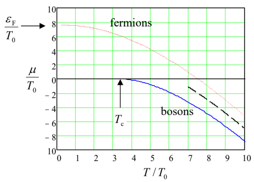
and then use this relation to calculate the ratios $T/T_0$ and $\mu /T_0 \equiv (\mu /T) \times (T/T_0)$, as functions of $\mu /T$ numerically. After that, we may plot the results versus each other, now considering the first ratio as the argument. Figure $\PageIndex{1}$ below shows the resulting plots, for both particle types. They show that at high temperatures, $T >> T_0$, the chemical potential is negative and approaches the classical behavior given by Equation ($\ref{46}$) for both fermions and bosons – just as we could expect. However, at temperatures $T \sim T_0$ the type of statistics becomes crucial. For fermions, the reduction of temperature leads to $\mu$ changing its sign from negative to positive, and then approaching a constant positive value called the Fermi energy, $\varepsilon_F \approx 7.595 \ T_0$ at $T \rightarrow 0$. On the contrary, the chemical potential of a bosonic gas stays negative, and then turns into zero at a certain critical temperature $T_c \approx 3.313 \ T_0$. Both these limits, which are very important for applications, may (and will be :-) explored analytically, separately for each statistics.

Figure $\PageIndex{1}$: The chemical potential of an ideal gas of $N >> 1$ indistinguishable quantum particles, as a function of temperature at a fixed gas density $n \equiv N/V$ (i.e. fixed $T_0 \propto n^{2/3})$, for two different particle types. The dashed line shows the classical approximation ($\ref{46}$), valid only at $T >> T_0$.

Before carrying out such studies (in the next two sections), let me show that, rather surprisingly, for any non-relativistic, ideal quantum gas, the relation between the product $PV$ and the energy,

Ideal gas: $\mathbf{PV}$ vs. $\mathbf{E}$

$$\boxed{PV = \frac{2}{3}E,}\label{48}$$

is exactly the same as follows from Eqs. ($3.1.19$) and ($3.1.20$) for the classical gas, and hence does not depend on the particle statistics. To prove this, it is sufficient to use Eqs. ($2.8.4$) and ($2.8.7$) for the grand thermodynamic potential of each quantum state, which may be conveniently represented by a single formula,

$$\Omega_k = \mp T \ln \left(1\pm e^{(\mu-\varepsilon_k)/T}\right),\label{49}$$

and sum them over all states $k$, using the general summation formula ($3.1.13$). The result for the total grand potential of a 3D gas with the dispersion law ($3.1.3$) is

$$\Omega=\mp T \frac{g V}{(2 \pi \hbar)^{3}} \int_{0}^{\infty} \ln \left(1 \pm e^{\left(\mu-p^{2} / 2 m\right) / T}\right) 4 \pi p^{2} d p=\mp T \frac{g V m^{3 / 2}}{\sqrt{2} \pi^{2} \hbar^{3}} \int_{0}^{\infty} \ln \left(1 \pm e^{(\mu-\varepsilon) / T}\right) \varepsilon^{1 / 2} d \varepsilon . \label{50}$$

Working out this integral by parts, exactly as we did it with the one in Equation ($2.6.10$), we get

$$\Omega=-\frac{2}{3} \frac{g V m^{3 / 2}}{\sqrt{2} \pi^{2} \hbar^{3}} \int_{0}^{\infty} \frac{\varepsilon^{3 / 2} d \varepsilon}{e^{(\varepsilon-\mu) / T} \pm 1}=-\frac{2}{3} \int_{0}^{\infty} \varepsilon g_{3}(\varepsilon)\langle N(\varepsilon)\rangle d \varepsilon . \label{51}$$

But the last integral is just the total energy $E$ of the gas:

Ideal gas: energy

$$\boxed{E=\frac{g V}{(2 \pi \hbar)^{3}} \int_{0}^{\infty} \frac{p^{2}}{2 m} \frac{4 \pi p^{2} d p}{e^{[\varepsilon(p)-\mu] / T} \pm 1}=\frac{g V m^{3 / 2}}{\sqrt{2} \pi^{2} \hbar^{3}} \int_{0}^{\infty} \frac{\varepsilon^{3 / 2} d \varepsilon}{e^{(\varepsilon-\mu) / T} \pm 1}=\int_{0}^{\infty} \varepsilon g_{3}(\varepsilon)\langle N(\varepsilon)\rangle d \varepsilon ,} \label{52}$$

so that for any temperature and any particle type, $\Omega = –(2/3)E$. But since, from thermodynamics, $\Omega = – PV$, we have Equation ($\ref{48}$) proved. This universal relation²² will be repeatedly used below.