3.3: Degenerate Fermi gas

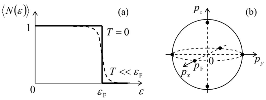
Analysis of low-temperature properties of a Fermi gas is very simple in the limit \(T = 0\). Indeed, in this limit, the Fermi-Dirac distribution (\(2.8.5\)) is just the step function:

\[\langle N(\varepsilon ) \rangle = \begin{cases} 1, & \text{ for } \varepsilon < \mu, \\ 0, & \text{ for } \mu < \varepsilon, \end{cases} \label{53}\]

- see by the bold line in Figure \(\PageIndex{1a}\). Since \(\varepsilon = p^2/2m\) is isotropic in the momentum space, in that space the particles, at \(T = 0\), fully occupy all possible quantum states inside a sphere (frequently called either the Fermi sphere or the Fermi sea) with some radius \(p_F\) (Figure \(\PageIndex{1b}\)), while all states above the sea surface are empty. Such degenerate Fermi gas is a striking manifestation of the Pauli principle: though in thermodynamic equilibrium at \(T = 0\) all particles try to lower their energies as much as possible, only \(g\) of them may occupy each translational (“orbital”) quantum state. As a result, the sphere’s volume is proportional to the particle number \(N\), or rather to their density \(n = N/V\).

Figure \(\PageIndex{1}\): Representations of the Fermi sea: (a) on the Fermi distribution plot, and (b) in the momentum space.

Indeed, the radius \(p_F\) may be readily related to the number of particles \(N\) using Equation (\(3.2.10\)), with the upper sign, whose integral in this limit is just the Fermi sphere’s volume:

\[N = \frac{gV}{(2\pi\hbar)^{3}} \int^{p_F}_0 4\pi p^2 dp = \frac{gV}{(2\pi\hbar)^{3}} \frac{4\pi}{3}p_F^3. \label{54}\]

Now we can use Equation (\(3.1.3\)) to express via \(N\) the chemical potential \(\mu\) (which, in the limit \(T = 0\), it bears the special name of the Fermi energy \(\varepsilon_F\))²³:

Fermi energy:

\[\boxed{ \varepsilon_F \equiv \mu\mid_{T=0} = \frac{p_F^2}{2m} = \frac{\hbar^2}{2m} \left( 6\pi^2 \frac{N}{gV}\right)^{2/3} \equiv \left(\frac{9\pi^{4}}{2}\right)^{1/3} T_0 \approx 7.595 T_0, } \label{55a}\]

where \(T_0\) is the quantum temperature scale defined by Equation (\(3.2.6\)). This formula quantifies the low temperature trend of the function \(\mu (T)\), clearly visible in Figure \(3.2.1\), and in particular, explains the ratio \(\varepsilon_F/T_0\) mentioned in Sec. 2. Note also a simple and very useful relation,

\[ \varepsilon_F = \frac{3}{2}\frac{N}{g_3 (\varepsilon_F)}, \quad \text{ i.e. }g_3 (\varepsilon_F) = \frac{3}{2} \frac{N}{\varepsilon_F},\label{55b}\]

that may be obtained immediately from the comparison of Eqs. (\(3.2.14\)) and (\ref{54}).

The total energy of the degenerate Fermi gas may be (equally easily) calculated from Equation (\(3.2.23\)):

\[E = \frac{gV}{(2\pi\hbar)^3} \int^{p_F}_0 \frac{p^2}{2m} 4\pi p^2 dp = \frac{gV}{(2\pi\hbar)^{3}} \frac{4\pi}{2m} \frac{p_F^5}{5} = \frac{3}{5} \varepsilon_F N, \label{56}\]

showing that the average energy, \(\langle \varepsilon \rangle \equiv E/N\), of a particle inside the Fermi sea is equal to 3/5 of that (\(\varepsilon_F\)) of the particles in the most energetic occupied states, on the Fermi surface. Since, according to the formulas of Chapter 1, at zero temperature \(H = G = N\mu \), and \(F = E\), the only thermodynamic variable still to be calculated is the gas pressure \(P\). For it, we could use any of the thermodynamic relations \(P = (H – E)/V\) or \(P = –(\partial F/\partial V)_T\), but it is even easier to use our recent result (\(3.2.19\)). Together with Equation (\ref{56}), it yields

\[ P = \frac{2}{3} \frac{E}{V} = \frac{2}{5} \varepsilon_F \frac{N}{V} = \left(\frac{36\pi^4}{125}\right)^{1/3} P_0 \approx 3.035 P_0, \quad \text{ where } P_0 \equiv nT_0 = \frac{\hbar^2n^{5/3}}{mg^{2/3}}. \label{57}\]

From here, it is straightforward to calculate the bulk modulus (reciprocal compressibility),²⁴

\[K \equiv -V \left(\frac{\partial P}{\partial V}\right)_T = \frac{2}{3} \varepsilon_F \frac{N}{V}, \label{58}\]

which may be simpler to measure experimentally than \(P\).

Perhaps the most important example²⁵ of the degenerate Fermi gas is the conduction electrons in metals – the electrons that belong to outer shells of the isolated atoms but become shared in solid metals, and as a result, can move through the crystal lattice almost freely. Though the electrons (which are fermions with spin \(s = 1/2\) and hence with the spin degeneracy \(g = 2s + 1 = 2\)) are negatively charged, the Coulomb interaction of the conduction electrons with each other is substantially compensated by the positively charged ions of the atomic lattice, so that they follow the simple model discussed above, in which the interaction is disregarded, reasonably well. This is especially true for alkali metals (forming Group 1 of the periodic table of elements), whose experimentally measured Fermi surfaces are spherical within 1% – even within 0.1% for Na.

Metal	\(\varepsilon_F\) (eV) Equation (\ref{55a}-\ref{55b})	\(K\) (GPa) Equation (\ref{58})	\(K\) (GPa) experiment	\(\gamma\)(mcal/mole\(\cdot\)K\(^2\)) Equation (\ref{69})	\(\gamma\)(mcal/mole\(\cdot\)K\(^2\)) experiment
Na	3.24	923	642	0.26	0.35
K	2.12	319	281	0.40	0.47
Rb	1.85	230	192	0.46	0.58
Cs	1.59	154	143	0.53	0.77

Looking at the values of \(\varepsilon_F\) listed in this table, note that room temperatures (\(T_K \sim 300\) K) correspond to \(T \sim 25\) meV. As a result, virtually all experiments with metals, at least in their solid or liquid form, are performed in the limit \(T << \varepsilon_F\). According to Equation (\(3.2.10\)), at such temperatures, the occupancy step described by the Fermi-Dirac distribution has a non-zero but relatively small width of the order of \(T\) – see the dashed line in Figure \(\PageIndex{1a}\). Calculations for this case are much facilitated by the so

called Sommerfeld expansion formula²⁹ for the integrals like those in Eqs. (\(3.2.12\)) and (\(3.2.23\)):

Sommerfeld expansion:

\[\boxed{I(T) \equiv \int^{\infty}_{0} \varphi (\varepsilon) \langle N (\varepsilon)\rangle d\varepsilon \approx \int^{\mu}_0 \varphi (\varepsilon) d\varepsilon + \frac{\pi^2}{6} T^2 \frac{d\varphi (\mu )}{d\mu}, \text{ for } T<<\mu,} \label{59}\]

where \(\phi (\varepsilon )\) is an arbitrary function that is sufficiently smooth at \(\varepsilon = \mu\) and integrable at \(\varepsilon = 0\). To prove this formula, let us introduce another function,

\[f(\varepsilon) \equiv \int^{\varepsilon}_0 \varphi (\varepsilon ' ) d\varepsilon', \quad \text{ so that } \varphi (\varepsilon ) = \frac{df( \varepsilon )}{d\varepsilon }, \label{60}\]

and work out the integral \(I(T)\) by parts:

\[I(T) \equiv \int^{\infty}_0 \frac{df(\varepsilon )}{d\varepsilon } \langle N(\varepsilon )\rangle d \varepsilon = \int^{\varepsilon = \infty}_{\varepsilon = 0} \langle N(\varepsilon)\rangle df \\ = [\langle N(\varepsilon)\rangle f(\varepsilon)]^{\varepsilon = \infty}_{\varepsilon =0} - \int^{\varepsilon = \infty}_{\varepsilon} f(\varepsilon ) d \langle N(\varepsilon)\rangle = \int^{\infty}_0 f(\varepsilon ) \left[ - \frac{\partial \langle N(\varepsilon)\rangle}{\partial \varepsilon} \right] d \varepsilon . \label{61}\]

As evident from Equation (\(2.8.5\)) and/or Figure \(\PageIndex{1a}\), at \(T << \mu\) the function \(–\partial \langle N(\varepsilon )\rangle /\partial \varepsilon\) is close to zero for all energies, besides a narrow peak of the unit area, at \(\varepsilon \approx \mu \). Hence, if we expand the function \(f(\varepsilon )\) in the Taylor series near this point, just a few leading terms of the expansion should give us a good approximation:

\[\begin{align} I(T) \approx & \int_{0}^{\infty}\left[f(\mu)+\left.\frac{d f}{d \varepsilon}\right|_{\varepsilon=\mu}(\varepsilon-\mu)+\left.\frac{1}{2} \frac{d^{2} f}{d \varepsilon^{2}}\right|_{\varepsilon=\mu}(\varepsilon-\mu)^{2}\right]\left[-\frac{\partial\langle N(\varepsilon)\rangle}{\partial \varepsilon}\right] d \varepsilon \nonumber\\ =& \int_{0}^{\mu} \varphi\left(\varepsilon^{\prime}\right) d \varepsilon^{\prime} \int_{0}^{\infty}\left(-\frac{\partial\langle N(\varepsilon)\rangle}{\partial \varepsilon}\right) d \varepsilon+\varphi(\mu) \int_{0}^{\infty}(\varepsilon-\mu)\left[-\frac{\partial\langle N(\varepsilon)\rangle}{\partial \varepsilon}\right] d \varepsilon \nonumber\\ &+\frac{1}{2} \frac{d \varphi(\mu)}{d \mu} \int_{0}^{\infty}(\varepsilon-\mu)^{2}\left[-\frac{\partial\langle N(\varepsilon)\rangle}{\partial \varepsilon}\right] d \varepsilon . \label{62}\end{align}\]

\[\int_{0}^{\infty}(\varepsilon-\mu)^{2}\left[-\frac{\partial\langle N(\varepsilon)\rangle}{\partial \varepsilon}\right] d \varepsilon \approx T^{2} \int_{-\infty}^{+\infty} \xi^{2} \frac{d}{d \xi}\left(-\frac{1}{e^{\xi}+1}\right) d \xi=4 T^{2} \int_{0}^{+\infty} \frac{\xi d \xi}{e^{\xi}+1}=4 T^{2} \frac{\pi^{2}}{12}. \label{63}\]

Being plugged into Equation (\ref{62}), this result proves the Sommerfeld formula (\ref{59}).

The last preparatory step we need to make is to account for a possible small difference (as we will see below, also proportional to \(T^2\)) between the temperature-dependent chemical potential \(\mu (T)\) and the Fermi energy defined as \(\varepsilon_F \equiv \mu (0)\), in the largest (first) term on the right-hand side of Equation (\ref{59}), to write

\[ I(T) \approx \int_{0}^{\varepsilon_{\mathrm{F}}} \varphi(\varepsilon) d \varepsilon+\left(\mu-\varepsilon_{\mathrm{F}}\right) \varphi(\mu)+\frac{\pi^{2}}{6} T^{2} \frac{d \varphi(\mu)}{d \mu} \equiv I(0)+\left(\mu-\varepsilon_{\mathrm{F}}\right) \varphi(\mu)+\frac{\pi^{2}}{6} T^{2} \frac{d \varphi(\mu)}{d \mu}. \label{64}\]

Now, applying this formula to Equation (\(3.2.12\)) and the last form of Equation (\(3.2.23\)), we get the following results (which are valid for any dispersion law \(\varepsilon (\mathbf{p})\) and even any dimensionality of the gas):

\[N(T) = N(0) + (\mu - \varepsilon_F) g(\mu) + \frac{\pi^2}{6} T^2 \frac{dg (\mu )}{d\mu}, \label{65}\]

\[E(T) = E(0) + (\mu - \varepsilon_F) \mu g(\mu) + \frac{\pi^2}{6} T^2 \frac{d}{d\mu}[\mu g (\mu )]. \label{66}\]

If the number of particles does not change with temperature, \(N(T) = N(0)\), as in most experiments, Equation (\ref{65}) gives the following formula for finding the temperature-induced change of \(\mu \):

\[\mu - \varepsilon_F = - \frac{\pi^2}{6} T^2 \frac{1}{g(\mu )} \frac{dg(\mu)}{d\mu}.\label{67}\]

Note that the change is quadratic in \(T\) and negative, in agreement with the numerical results shown with the red line in Figure \(3.2.1\). Plugging this expression (which is only valid when the magnitude of the change is much smaller than \(\varepsilon_F\)) into Equation (\ref{66}), we get the following temperature correction to the energy:

\[E(T)-E(0) = \frac{\pi^2}{6} g(\mu)T^2, \label{68}\]

where within the accuracy of our approximation, \(\mu\) may be replaced with \(\varepsilon_F\). (Due to the universal relation (\(3.2.19\)), this result also gives the temperature correction to the Fermi gas’ pressure.) Now we may use Equation (\ref{68}) to calculate the heat capacity of the degenerate Fermi gas:

Low-T heat capacity:

\[\boxed{C_V \equiv \left(\frac{\partial E}{\partial T } \right)_V = \gamma T, \quad \text{ with } \gamma = \frac{\pi^2}{3} g(\varepsilon_F).} \label{69}\]

According to Equation (\ref{55b}), in the particular case of a 3D gas with the isotropic and parabolic dispersion law (\(3.1.3\)), Equation (\ref{69}) reduces to

\[\gamma = \frac{\pi^2}{2} \frac{N}{\varepsilon_F}, \quad \text{ i.e. } c_V \equiv \frac{C_V}{N} = \frac{\pi^2}{2} \frac{T}{\varepsilon_F} << 1. \label{70}\]

This important result deserves a discussion. First, note that within the range of validity of the Sommerfeld approximation (\(T << \varepsilon_F\)), the specific heat of the degenerate gas is much smaller than that of the classical gas, even without internal degrees of freedom: \(c_V = 3/2\) – see Equation (\(3.1.20\)). The physical reason for such a low heat capacity is that the particles deep inside the Fermi sea cannot pick up thermal excitations with available energies of the order of \(T << \varepsilon_F\), because the states immediately above them are already occupied. The only particles (or rather quantum states, due to the particle indistinguishability) that may be excited with such small energies are those at the Fermi surface, more exactly within a surface layer of thickness \(\Delta \varepsilon \sim T << \varepsilon_F\), and Equation (\ref{70}) presents a very vivid manifestation of this fact.

The second important feature of Eqs. (\ref{69})-(\ref{70}) is the linear dependence of the heat capacity on temperature, which decreases with a reduction of \(T\) much slower than that of crystal vibrations – see Equation (\(2.6.21\)). This means that in metals the specific heat at temperatures \(T << T_D\) is dominated by the conduction electrons. Indeed, experiments confirm not only the linear dependence (\ref{70}) of the specific heat,³¹ but also the values of the proportionality coefficient \(\gamma \equiv C_V/T\) for cases when \(\varepsilon_F\) can be calculated independently, for example for alkali metals – see the two rightmost columns of Table 1 above. More typically, Equation (\ref{69}) is used for the experimental measurement of the density of states on the Fermi surface, \(g(\varepsilon_F)\) – the factor which participates in many theoretical results, in particular in transport properties of degenerate Fermi gases (see Chapter 6 below).