21.6: Applications

In this section, we briefly outline a few applications of the magnetic force.

Velocity selector and mass spectrometer

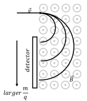
In Example 21.2.1, we described how charged particles with different charge-to-mass ratios will undergo uniform circular motion with different radii, if they all have the same speed. This principle is used in mass spectrometers, which are devices that are able to detect trace amounts of matter in a sample. For example, when your bag gets swiped with a sticky tape at a security check at the airport, that piece of sticky tape is then analyzed by a mass spectrometer.

The tape is vaporized in a way to ionize the atoms on the tape. The ions are then accelerated through an electric potential difference and then pass through a region with a magnetic field. The ions typically execute half of a circular orbit before being detected, as illustrated in Figure \(\PageIndex{1}\). The charge-to-mass ratio of the ions is determined from the radius of their orbit. Usually, their charge is either one or two times the electron charge, allowing their mass to be determined.

Figure \(\PageIndex{1}\): Illustration of how a mass spectrometer can separate ions based on their charge-to-mass ratio. A detector is placed to measure the number of ions that appear at each radius, allowing the composition of a sample to be determined.

In order for the mass spectrometer to function as designed, it is important that all of the charged particles enter the region of magnetic field with the same speed. A velocity selector is a device that combines perpendicular electric and magnetic fields in order to select only particles of a certain speed, regardless of their mass. The velocity selector is illustrated in Figure \(\PageIndex{2}\)

Figure \(\PageIndex{2}\): Illustration of a velocity selector. Only charged particles with a specific speed can make it through without colliding with one of the plates.

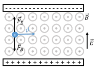
In a velocity selector, both an electric and a magnetic force are exerted. Figure \(\PageIndex{2}\) shows a positive particle moving toward the right with speed, \(v\). The particle will experience an upwards electric force and a downwards magnetic force. If those two forces are equal, then the particle will move in a straight line. If, instead, one of the forces is larger than the other, the particle will be deflected and hit one of the charged plates. The condition for the two forces to be equal is given by:

\[\begin{aligned} F_B &= F_E\\[4pt] qvB &= qE\\[4pt] \therefore v=\frac{E}{B}\end{aligned}\]

Thus, the electric and magnetic fields can be tuned so that their ratio gives the desired speed. Note that the speed selector works regardless of the sign of the charge or its mass, which makes it ideal to filter the particles entering a mass spectrometer.

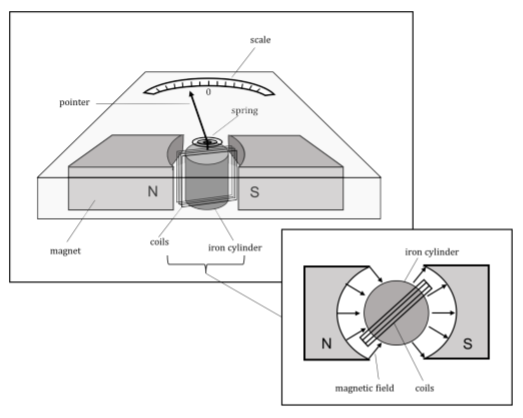
Galvanometer

The galvanometer makes use of the magnetic force in order to measure electric current. In a galvanometer, a coil (many loops) is placed in a known magnetic field. As current passes through the coil, the magnetic dipole moment of the coil increases, and the magnetic field exerts a torque on the coil. The torque from the magnetic force is balanced by the restoring torque of a torsional spring (a coil spring). A needle is attached to the coil, and the deflection of the needle, proportional to the current in the coil, is then a measure of the current through the coil. A galvanometer is illustrated in Figure \(\PageIndex{3}\).

Figure \(\PageIndex{3}\): Illustration of a galvanometer. Current passes through the coil, and the coil rotates due to the torque from a magnetic field created by a permanent magnet. The torque from the magnetic force is balanced by a torsional spring.​​​​​​​

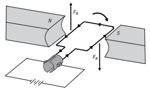
Electric motor

In an electric motor, a current-carrying coil (many loops) is immersed in a fixed and uniform magnetic field. As current passes through the coil, the coil experiences a torque and rotates. Once the coil has reached a position where its magnetic dipole moment vector is parallel to the magnetic field, the direction of the current is reversed, so that the coil continues to feel a torque for another half turn, until the direction of the current is reversed again. This is illustrated in Figure \(\PageIndex{4}\).

Figure \(\PageIndex{4}\): Illustration of a DC electric motor. Current circulates in the coil resulting in a torque from the magnetic field. Once the coil is aligned with the magnetic field, the direction of the current in the coil is inverted, so that the coil continues to feel a torque. The current is inverted using mechanical brushes that reverse the leads on the coil every half turn.​​​​​​​

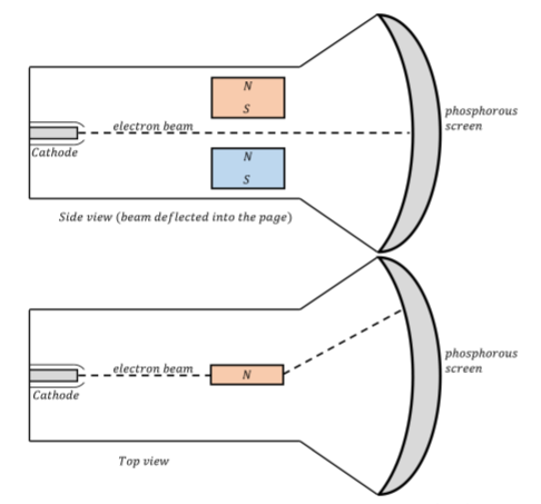
Cathode ray tube

The cathode ray tube is the main component of old televisions and monitors. In those devices, a beam of electrons is accelerated by an electric potential difference. The electrons then hit a phosphorescent screen, that emits light when the electrons collide with the screen. A magnetic field is used to deflect the electron beam to different parts of the screen and create the desired image, in a rapid sweeping motion, fast enough that the human eye cannot detect the sweeping motion. An example of a cathode ray tube is shown in Figure \(\PageIndex{5}\).

Figure \(\PageIndex{5}\): Illustration of a cathode ray tube from a side view (top) and a top view (bottom). A magnetic field is used to deflect a beam of electrons onto a screen. The perpendicular magnetic fields are used to sweep the beam rapidly across the whole screen to create an image​​​​​​​.

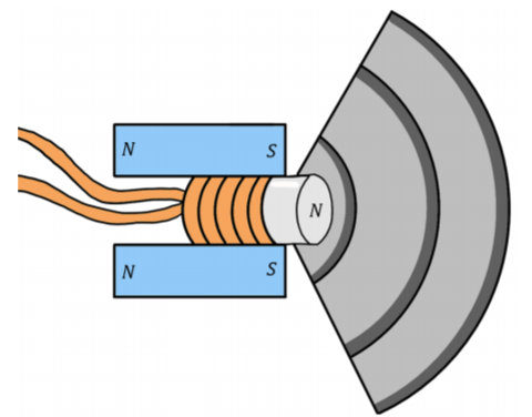
Loudspeaker

In a loudspeaker, a coil is immersed in a non-uniform magnetic field. The coil is attached to a membrane so that the membrane moves with the coil when a magnetic force is exerted on the coil. AC current circulates in the coil, with the same frequencies as the desired sound. The coil then moves at those frequencies and the membrane then displaces the air, creating the desired sound waves.

Figure \(\PageIndex{6}\): Illustration of a loud speaker. As current moves through the coil, the coil is pushed back and forth by the magnetic force exerted by a permanent magnet. The motion is transferred to a membrane that move the air and creates the sound wave.​​​​​​​​​​​​​​