16.8: Problems

Last updated
Save as PDF

Page ID: 33214

\( \newcommand{\vecs}[1]{\overset { \scriptstyle \rightharpoonup} {\mathbf{#1}} } \) \( \newcommand{\vecd}[1]{\overset{-\!-\!\rightharpoonup}{\vphantom{a}\smash {#1}}} \)\(\newcommand{\id}{\mathrm{id}}\) \( \newcommand{\Span}{\mathrm{span}}\) \( \newcommand{\kernel}{\mathrm{null}\,}\) \( \newcommand{\range}{\mathrm{range}\,}\) \( \newcommand{\RealPart}{\mathrm{Re}}\) \( \newcommand{\ImaginaryPart}{\mathrm{Im}}\) \( \newcommand{\Argument}{\mathrm{Arg}}\) \( \newcommand{\norm}[1]{\| #1 \|}\) \( \newcommand{\inner}[2]{\langle #1, #2 \rangle}\) \( \newcommand{\Span}{\mathrm{span}}\) \(\newcommand{\id}{\mathrm{id}}\) \( \newcommand{\Span}{\mathrm{span}}\) \( \newcommand{\kernel}{\mathrm{null}\,}\) \( \newcommand{\range}{\mathrm{range}\,}\) \( \newcommand{\RealPart}{\mathrm{Re}}\) \( \newcommand{\ImaginaryPart}{\mathrm{Im}}\) \( \newcommand{\Argument}{\mathrm{Arg}}\) \( \newcommand{\norm}[1]{\| #1 \|}\) \( \newcommand{\inner}[2]{\langle #1, #2 \rangle}\) \( \newcommand{\Span}{\mathrm{span}}\)\(\newcommand{\AA}{\unicode[.8,0]{x212B}}\)

Imagine that an electron actually consists of two point charges, each with charge \(e / 2,\), separated by a distance \(D\), where \(e\) is the charge on the electron. Compute \(D\) such that the potential energy of the two charges equals the rest energy of the electron. Look up the constants and compute a numerical value for \(D\). Finally, compute the force between the two charges and compare to the gravitational force between two masses each equal to half the electron mass separated by this distance.
Verify that the equations for the scalar potentials associated with a sheet and a line of charge, (16.8) and (16.10), yield the corresponding electric fields.
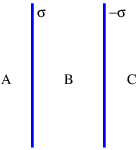
Two sheets of charge, one with charge density \(\sigma\), the other with -\(\sigma\), are aligned as shown in figure 16.10. Compute the electric field in each of the regions A, B, and C.
Figure 16.10: Two parallel sheets of charge, one with surface charge density \(σ\), the other with -\(σ\).
_____________________________________
Positive charge is distributed uniformly on the upper surface of an infinite conducting plate with charge per unit area \(\sigma\) as shown in figure 16.11. Use Gauss’s law to compute the electric field above the plate. Hint: Is there any electric field inside the plate?
Figure 16.11: A charged metal plate.
_____________________________________
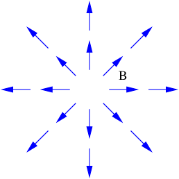
Suppose a student proposes that a magnetic field can take the form shown in figure 16.12. Is the proposed form of the magnetic field consistent with Gauss’s law for magnetism? Explain.
Figure 16.12: Hypothesized magnetic field. Does it satisfy Gauss’s law for magnetism?
_____________________________________
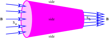
The magnetic flux through the sides of the cone illustrated in figure 16.13 is zero. The magnetic field may be assumed to be approximately normal to the ends of the cone and the magnetic flux into the left end is Φ_B. The areas of the left and right ends of the cone are \(S\)_a and \(S\)_b.
Figure 16.13: Converging magnetic field passing through a closed surface.
_____________________________________
1. What is the magnetic flux out of the right end of the cone?
2. What is the value of the magnetic field \(B\) on the left end of the cone?
3. What is the value of \(B\) on the right end?
In the lab frame a wire has negative charge with linear charge density -\(\lambda\) moving at speed -\(U\) corresponding to a current \(i\) = \(λU \) as shown in figure 16.14. Positive charge is stationary, and has charge density \(\lambda\), so the net charge is zero.
1. What are the electric and magnetic fields produced by the charge in the wire in the stationary frame?
2. In a reference frame moving at velocity -\(U\) in the \(x\) direction, such that the negative charge is stationary, what is the apparent linear charge density of (1) the negative charge, and (2) the positive charge? Hint: The Lorentz contraction must be taken into account here.
3. What is the electric field produced by the charge in the wire in the moving frame? Hint: Do the charge densities from the positive and negative charge cancel in this frame?
4. What is the current in the wire in the moving frame, and hence, what is the magnetic field around the wire in this frame? Hint: Is the positive or negative charge causing the current in this frame?
5. Explain why the net force on a separate charged particle some distance from the wire and stationary in the lab frame is zero in both reference frames. Figure 16.14: A horizontal wire with current \(i \) viewed in two different reference frames.
  _____________________________________
The left panel of figure 16.8 shows a real charged particle A emitting a real photon, turning into a possibly different real particle B after the emission. If particle A and particle B have the same mass, show that this process is energetically impossible. Hint: Work in a reference frame in which particle A is stationary.
Given the four-potential for an electromagnetic plane wave, show why the longitudinal component of the magnetic field is zero.
Referring to figure 16.9, show that the vector \(\mathbf{E} \times \mathbf{B}\) points in the direction of propagation of a plane electromagnetic wave.
Referring to figure 16.9, what direction and speed must a charged particle move in the presence of a free electromagnetic wave such that the net electromagnetic force on the particle is zero?