17.5: Kirchhoff’s Laws

Last updated
Save as PDF

Page ID: 32853

\( \newcommand{\vecs}[1]{\overset { \scriptstyle \rightharpoonup} {\mathbf{#1}} } \) \( \newcommand{\vecd}[1]{\overset{-\!-\!\rightharpoonup}{\vphantom{a}\smash {#1}}} \)\(\newcommand{\id}{\mathrm{id}}\) \( \newcommand{\Span}{\mathrm{span}}\) \( \newcommand{\kernel}{\mathrm{null}\,}\) \( \newcommand{\range}{\mathrm{range}\,}\) \( \newcommand{\RealPart}{\mathrm{Re}}\) \( \newcommand{\ImaginaryPart}{\mathrm{Im}}\) \( \newcommand{\Argument}{\mathrm{Arg}}\) \( \newcommand{\norm}[1]{\| #1 \|}\) \( \newcommand{\inner}[2]{\langle #1, #2 \rangle}\) \( \newcommand{\Span}{\mathrm{span}}\) \(\newcommand{\id}{\mathrm{id}}\) \( \newcommand{\Span}{\mathrm{span}}\) \( \newcommand{\kernel}{\mathrm{null}\,}\) \( \newcommand{\range}{\mathrm{range}\,}\) \( \newcommand{\RealPart}{\mathrm{Re}}\) \( \newcommand{\ImaginaryPart}{\mathrm{Im}}\) \( \newcommand{\Argument}{\mathrm{Arg}}\) \( \newcommand{\norm}[1]{\| #1 \|}\) \( \newcommand{\inner}[2]{\langle #1, #2 \rangle}\) \( \newcommand{\Span}{\mathrm{span}}\)\(\newcommand{\AA}{\unicode[.8,0]{x212B}}\)

Figure 17.8: A typical circuit to which we apply Kirchhoff’s laws.

In the above discussion of energy we made two assumptions about electric circuits, which consist of electronic components connected by wires:

Currents are conserved. Thus, the current entering one end of a wire connecting two devices is equal to the current leaving the other end, and the current out of the generator in the left panel of figure 17.7 is assumed to equal the current into and out of the capacitor. No electric charge is stored in any of the wires connecting components.
The electric fields outside of components are conservative, and therefore are derived solely from the scalar potential. Thus, the net work done on a charged particle passing completely around a circuit loop is zero and the positive work done on charge passing through the generator in the right panel of figure 17.7 is exactly balanced by the potential difference across the inductor. As a result, the effects of electric fields outside of components can be represented by electrostatic potentials, or “voltages”. Every part of a wire connecting components has the same potential and the effect of each component is to maintain a potential difference between its input and output connections.

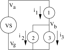
These are called Kirchhoff’s laws. They are used extensively in electronic circuit design. Figure 17.8 illustrates a typical circuit with a voltage source VS, which may be a battery or generator, and three circuit components. The voltage source provides a potential difference equal to \(V\)_a - \(V\) _g, which is equal simply to \(V\) _a, since we are assuming that \(V_g = 0\). (Since the scalar potential is insensitive to an arbitrary additive constant, we can always set the potential at one point in the circuit to zero to simplify our calculations.) The voltage drop across component 1 is \(V\) _a - \(V\) _b and the voltage drop across both components 2 and 3 is \(V\) _b - \(V\) _g. If the components are resistors, then Ohm’s law can be used to relate the voltage drops across the components to the currents through them. If they are capacitors or inductors, the voltage drop is related respectively to the charge on the capacitor or the time rate of change of current through the inductor. The time rate of change of the charge on the capacitor can be related to the current through the capacitor. The final point in figure 17.8 is that current is conserved at junctions, i. e., \(i\) ₁ = \(i\) ₂ + \(i\) ₃. The methods of algebra (for just resistors) or calculus (if there are capacitors or inductors) can then be used to calculate all currents and voltages.

It is important to realize that Kirchhoff’s laws are only approximations that hold when the currents and potentials in a circuit change slowly with time. For steady currents and constant potentials they are precisely true, since imbalances in charge entering and leaving a junction between devices would result in the indefinite buildup of charge in the junction with time and therefore an increasing electrostatic potential, which would violate the steady state assumption. Furthermore, a non-zero EMF around a closed loop would result in net acceleration of charge around the loop and a constantly increasing current.

If currents and potentials are changing with time, Kirchhoff’s laws are approximately valid only if the capacitance, inductance, and resistance of the wires connecting circuit elements are much smaller than the capacitance, inductance, and resistance of the circuit elements themselves. For very high frequency operation, the effects of these “parasitic” properties are not small and must be included in the design of the circuit.