2.3: Superposition of Plane Waves

We now study wave packets in two dimensions by asking what the superposition of two plane sine waves looks like. If the two waves have different wavenumbers, but their wave vectors point in the same direction, the results are identical to those presented in the previous chapter, except that the wave packets are indefinitely elongated without change in form in the direction perpendicular to the wave vector. The wave packets produced in this case move in the direction of the wave vectors and thus appear to a stationary observer like a series of passing pulses with broad lateral extent.

Superimposing two plane waves which have the same frequency results in a stationary wave packet through which the individual wave fronts pass. This wave packet is also elongated indefinitely in some direction, but the direction of elongation depends on the dispersion relation for the waves being considered. These wave packets are in the form of steady beams, which guide the individual phase waves in some direction, but don’t themselves change with time. By superimposing multiple plane waves, all with the same frequency, one can actually produce a single stationary beam, just as one can produce an isolated pulse by superimposing multiple waves with wave vectors pointing in the same direction.

If the frequency of a wave depends on the magnitude of the wave vector, but not on its direction, the wave’s dispersion relation is called isotropic; otherwise it is anisotropic. In the isotropic case, two waves have the same frequency only if the lengths of their wave vectors, and hence their wavelengths, are the same. The first two examples in figure 2.6 satisfy this condition, while the last example is anisotropic.

Figure \(\PageIndex{2}\): .7: Wave fronts and wave vectors (k₁ and k₂) of two plane waves with the same wavelength but oriented in different directions. The vertical bands show regions of constructive interference where wave fronts coincide. The vertical regions in between have destructive interference, and hence define the lateral boundaries of the beams produced by the superposition. The quantities k₀ and Δk are also shown.

Figure \(\PageIndex{2}\): .8: Example of beams produced by two plane waves with the same wavelength moving in different directions. The wave vectors of the two waves are k = (±0.1, 1.0). Regions of positive displacement are lighter, while regions of negative displacement are darker.

We now use the language of vectors to investigate the superposition of two plane waves with wave vectors k₁ and k₂:

\[h=\sin \left(\mathbf{k}_{1} \cdot \mathbf{x}-\omega t\right)+\sin \left(\mathbf{k}_{2} \cdot \mathbf{x}-\omega t\right)\label{2.15}\]

Applying the trigonometric identity for the sine of the sum of two angles (as we have done previously), equation (\ref{2.15}) can be reduced to

\[h=2 \sin \left(\mathbf{k}_{0} \cdot \mathbf{x}-\omega t\right) \cos (\Delta \mathbf{k} \cdot x)\label{2.16}\]

where

\[\mathbf{k}_{0}=\left(\mathbf{k}_{1}+\mathbf{k}_{2}\right) / 2 \quad \Delta \mathbf{k}=\left(\mathbf{k}_{2}-\mathbf{k}_{1}\right) / 2\label{2.17}\]

This is in the form of a sine wave moving in the k₀ direction with phase speed \(c_{\text {phase }}=\omega / |\mathbf{k}_{0}|\) and wavenumber \(\left|\mathbf{k}_{0}\right|\), modulated in the Δk direction by a cosine function. The lines of destructive interference are normal to Δk. The distance w between lines of destructive interference is the distance between successive zeros of the cosine function in equation (\ref{2.16}), implying that \(|\Delta \mathbf{k}| w=\pi\), which leads to

\[w=\pi /|\Delta \mathbf{k}|\label{2.18}\]

Thus, the smaller \(|\Delta \mathbf{k}|\) the greater is the beam diameter.

Waves of Identical Wavelength

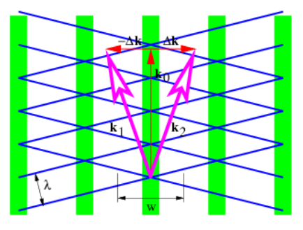
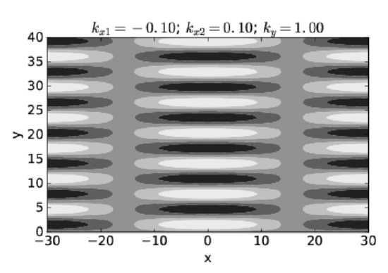
In this section we investigate the beams produced by superimposing isotropic waves of the same frequency. Figure 2.7 illustrates what happens in such a superposition. Vectors k₁ and k₂ of equal length give rise to a mean wave vector k₀ and half the difference, Δk. As illustrated, the lines of constructive and destructive interference are perpendicular to Δk. Figure 2.8 shows a concrete example of the beams produced by superposition of two plane waves of equal wavelength oriented as in figure 2.7. The beams are aligned vertically, since Δk is horizontal, with the lines of destructive interference separating the beams located near x = ±16. The transverse width of the beams of ≈ 32 satisfies equation (\ref{2.18}) with |Δk| = 0.1. Each beam is made up of vertically propagating phase waves, with the crests and troughs indicated by the regions of white and black.

Waves of Differing Wavelength

In the third example of figure 2.6, the frequency of the wave depends only on the direction of the wave vector, independent of its magnitude, which is the reverse of the case for an isotropic dispersion relation. In this highly anisotropic case, different plane waves with the same frequency have wave vectors which point in the same direction, but have different lengths.

Figure \(\PageIndex{2}\): .9: Wave fronts and wave vectors (k₁ and k₂) of two plane waves with different wavelengths oriented in different directions. The slanted bands show regions of constructive interference where wave fronts coincide. The slanted regions in between have destructive interference, and as mentioned previously, define the lateral limits of the beams produced by the superposition. The quantities k₀ and Δk are also shown.

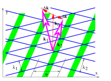
More generally, one might have waves for which the frequency depends on both the direction and magnitude of the wave vector. In this case, two different plane waves with the same frequency would typically have wave vectors which differ both in direction and magnitude. Such an example is illustrated in figures 2.9 and 2.10.

Figure \(\PageIndex{2}\): .10: Example of beams produced by two plane waves with wave vectors differing in both direction and magnitude. The wave vectors of the two waves are k₁ = (-0.1, 1.0) and k₂ = (0.1, 0.9). Regions of positive displacement are lighter, while regions of negative displacement darker.

Figure \(\PageIndex{2}\): .11: Illustration of factors entering the addition of two plane waves with the same frequency. 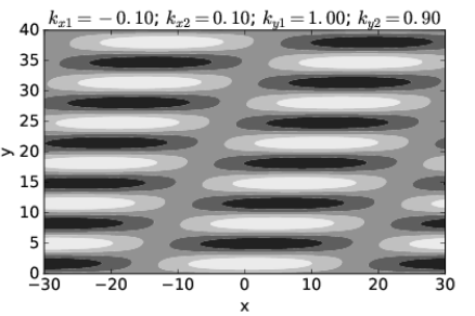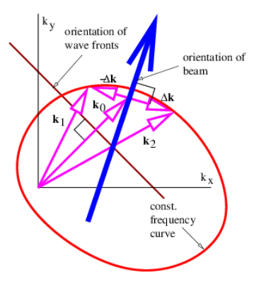The wave fronts are perpendicular to the vector average of the two wave vectors, \(\mathbf{k}_{0}=\left(\mathbf{k}_{1}+\mathbf{k}_{2}\right) / 2\), while the lines of constructive interference, which define the beam orientation, are oriented perpendicular to the difference between these two vectors, \(\Delta \mathbf{k}=\left(\mathbf{k}_{2}-\mathbf{k}_{1}\right) / 2\)

Figure 2.11 summarizes what we have learned about adding plane waves with the same frequency. In general, the beam orientation (and the lines of constructive interference) are not perpendicular to the wave fronts. This only occurs when the wave frequency is independent of wave vector direction.

Waves with the Same Wavelength

As with wave packets in one dimension, we can add together more than two waves to produce an isolated wave packet. We will confine our attention here to the case of an isotropic dispersion relation in which all the wave vectors for a given frequency are of the same length.

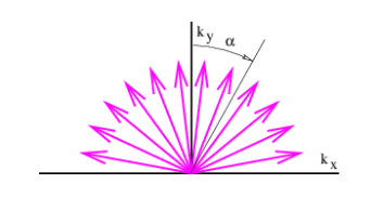
Figure \(\PageIndex{2}\): .12: Illustration of wave vectors of plane waves which might be added together.

Figure 2.12 shows an example of this in which wave vectors of the same wavelength but different directions are added together. Defining \(\alpha_{i}\) as the angle of the \(i_{th}\) wave vector clockwise from the vertical, as illustrated in figure 2.12, we could write the superposition of these waves at time t = 0 as

\[\begin{equation}
\begin{aligned}
h &=\sum_{i} h_{i} \sin \left(k_{x i} x+k_{y i} y\right) \\
&=\sum_{i} h_{i} \sin \left[k x \sin \left(\alpha_{i}\right)+k y \cos \left(\alpha_{i}\right)\right]
\end{aligned}
\end{equation}\label{2.19}\]

where we have assumed that \(k_{x i}=k \sin \left(\alpha_{i}\right) \text { and } k_{y i}=k \cos \left(\alpha_{i}\right)\). The parameter \(k=|\mathbf{k}|\) is the magnitude of the wave vector and is the same for all the waves. Let us also assume in this example that the amplitude of each wave component decreases with increasing \(\left|\alpha_{i}\right|:\).

\[h_{i}=\exp \left[-\left(\alpha_{i} / \alpha_{\max }\right)^{2}\right]\label{2.20}\]

The exponential function decreases rapidly as its argument becomes more negative, and for practical purposes, only wave vectors with \(\left|\alpha_{i}\right| \leq \alpha_{m a x}\) contribute significantly to the sum. We call \(\alpha_{\max }\) the spreading angle.

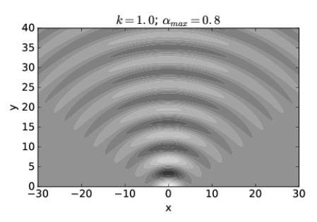
Figure \(\PageIndex{2}\): .13: Plot of the displacement field h (x,y) from equation (2.19) for α_max = 0.8 and k = 1.

Figure 2.13 shows what h(x,y) looks like when \(\alpha_{\max }=0.8\) radians and \(k = 1\). Notice that for y = 0 the wave amplitude is only large for a small region in the range \(-4 < x < 4\). However, for \(y > 0\) the wave spreads into a broad, semicircular pattern.

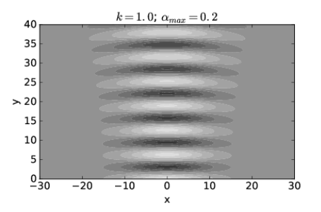
Figure \(\PageIndex{2}\): .14: Plot of the displacement field h (x,y) from equation (2.19) for \(\alpha_{\max }=0.2 \text { and } k=1\).

Figure 2.14 shows the computed pattern of h(x,y) when the spreading angle \(\alpha_{\max }=0.2\) radians. The wave amplitude is large for a much broader range of \(x\) at \(y = 0\) in this case, roughly \(-12 < x < 12\). On the other hand, the subsequent spread of the wave is much smaller than in the case of figure 2.13.

We conclude that a superposition of plane waves with wave vectors spread narrowly about a central wave vector which points in the y direction (as in figure 2.14) produces a beam which is initially broad in x but for which the breadth increases only slightly with increasing y. However, a superposition of plane waves with wave vectors spread more broadly (as in figure 2.13) produces a beam which is initially narrow in x but which rapidly increases in width as y increases.

The relationship between the spreading angle \(\alpha_{\max }\) and the initial breadth of the beam is made more understandable by comparison with the results for the two-wave superposition discussed at the beginning of this section. As indicated by equation (\ref{2.18}), large values of \(k_{x}\), and hence α, are associated with small wave packet dimensions in the x direction and vice versa. The superposition of two waves doesn’t capture the subsequent spread of the beam which occurs when many waves are superimposed, but it does lead to a rough quantitative relationship between α_max (which is just \(\tan ^{-1}\left(k_{t} / k_{y}\right)\) in the two wave case) and the initial breadth of the beam. If we invoke the small angle approximation for α = α_max so that \(\alpha_{\max }=\tan ^{-1}\left(k_{t} / k_{y}\right) \approx k_{t} / k_{y} \approx k_{t} k,\) then k_x ≈ kα_max and equation (\ref{2.18}) can be written \(w=\pi k_{x} \approx \pi\left(k \alpha_{\max }\right)=\lambda\left(2 \alpha_{\max }\right)\). Thus, we can find the approximate spreading angle from the wavelength of the wave λ and the initial breadth of the beam w:

\[\alpha_{\max } \approx \lambda /(2 w) \quad \text { (single slit spreading angle) }\label{2.21}\]