1.8: A Simple Nonlinear Oscillator

To illustrate some of the differences between linear and nonlinear oscillators, we will give one very simple example of a nonlinear oscillator. Consider the following nonlinear equation of motion:

\[m \frac{d^{2}}{d t^{2}} x=\left\{\begin{array}{l}-F_{0} \text { for } x>0 \\ F_{0} \text { for } x<0 \\ 0 \text { for } x=0\end{array}\right.\]

This describes a particle with mass, \(m\), that is subject to a force to the left, \(−F_0\), when the particle is to the right of the origin (\(x(t) > 0\)), a force to the right, \(F_0\), when the particle is to the left of the origin (\(x(t) < 0\)), and no force when the particle is sitting right on the origin. The potential energy for this system grows linearly on both sides of x = 0. It cannot be differentiated at \(x = 0\), because the derivative is not continuous there. Thus, we cannot expand the potential energy (or the force) in a Taylor series around the point \(x = 0\), and the arguments of (1.21)-(1.24) do not apply. It is easy to find a solution of (1.120). Suppose that at time, \(t = 0\), the particle is at the origin but moving with positive velocity, \(v\). The particle immediately moves to the right of the origin and decelerates with constant acceleration, \(\frac{−F_0}{m}\), so that

\[x(t) = vt - \frac{F_o}{2m}t^2\]

for \(t ≤ τ\).

where

\[τ=\frac{2mv}{F_o}\]

is the time required for the particle to turn around and get back to the origin. At time, \(t = τ\), the particle moves to the left of the origin. At this point it is moving with velocity, \(−v\), the process is repeated for negative \(x\) and positive acceleration \(\frac{F_0}{m}\) Then the solution continues in the form

\[x(t) = −v(t − τ ) + \frac{F_o}{2m}(t − τ )^2 for τ ≤ t ≤ 2τ\]

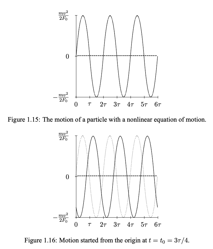
Then the whole process repeats. The motion of the particle, shown in figure 1.15, looks superficially like harmonic oscillation, but the curve is a sequence of parabolas pasted together, instead of a sine wave. The equation of motion, (1.120), is time translation invariant. Clearly, we can start the particle at the origin with velocity, v, at any time, t0. The solution then looks like that shown in figure 1.15 but translated in time by \(t_0\). The solution has the form

\[x_{t0}(t) = x(t-t_o)\]

where \(x(t)\) is the function described by (1.121), (1.123), etc. This shown in figure 1.16 for \(t = t_0 = \frac{3τ}{4}\). The dotted curve corresponds to \(t_0 = 0\)

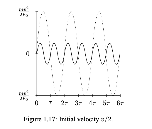
Like the harmonic oscillator, this system oscillates regularly and indefinitely. However, in this case, the period of the oscillation, the time it takes to repeat, 2τ , depends on the amplitude of the oscillation, or equivalently, on the initial velocity, v. The period is proportional to v, from (1.122). The motion of the particle started from the origin at \(t = t_0\), for an initial velocity v/2 is shown in figure 1.17. The dotted curve corresponds to an initial velocity, v. While the nonlinear equation of motion, (1.120), is time translation invariant, the symmetry is much less useful because the system lacks linearity. From our point of view, the important thing about linearity (apart from the fact that it is a good approximation in so many important physical systems), is that it allows us to choose a convenient basis for the solutions to the equation of motion. We choose them to behave simply under time translations.

Then, because of linearity, we can build up any solution as a linear combination of the basis solutions. In a situation like (1.120), we do not have this option.