11.1: The k Vector

Consider the two-dimensional beaded mesh, a two-dimensional analog of the beaded string, shown in Figure \( 11.1\). All the beads have mass \(m\). The tension of the horizontal (vertical) strings is \(T_{H}\) \((T_{V})\) and the interbead distance is \(a_{H}\) \((a_{V})\). There is no damping. We can label the beads by a pair of integers (\(j\), \(k\)) indicating their horizontal and vertical positions as shown. Alternatively, we can label the beads by their positions in the \(x\), \(y\) plane according to \[(x, y)=\left(j a_{H}, k a_{V}\right) .\]

Thus, we can describe their small transverse (out of the plane of the paper, in the \(z\) direction) oscillations either by a matrix \(\psi_{j k}(t)\) or by a function \[\psi(x, y, t) ; \quad 0 \leq x \leq 5 a_{H}, 0 \leq y \leq 4 a_{V} .\]

We will use (11.2) because we can then extend the discussion to continuous systems more easily. We are interested only in the transverse oscillations of this system, in which the blocks move up and down out of the plane of the paper, because these oscillations do not stretch the strings very much (only to second order in the small displacements). The other oscillations of such a system have much higher frequencies and are strongly damped, so they are not very interesting.

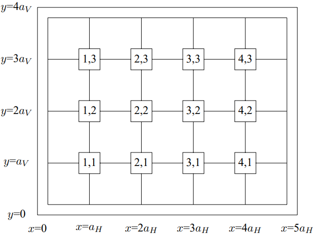
Figure \( 11.1\): A two-dimensional beaded mesh.

As in the one-dimensional case, the first step is to remove the walls and consider the infinite system obtained by extending the interior in all directions. The oscillations of the resulting system can be described by a function \(\psi(x, y, t)\), where \(x\) and \(y\) are not constrained.

This infinite system looks the same if it is translated by \(a_{V}\) vertically, or by \(a_{H}\) horizontally. We can write down solutions for the infinite system by using our discussion of the one-dimensional case twice. Because the system has translation invariance in the \(x\) direction, we expect that we can find eigenstates of the \(M^{−1}K\) matrix proportional to \[e^{i k_{x} x}\]

for any constant \(k_{x}\). Because the system has translation invariance in the \(y\) direction, we expect that we can find eigenstates of the \(M^{−1}K\) matrix proportional to \[e^{i k_{y} y}\]

for any constant \(k_{y}\). Putting (11.3) and (11.4) together, we expect that we can find eigenstates of the \(M^{−1}K\) matrix that have the form \[\psi(x, y)=A e^{i k_{x} x} e^{i k_{y} y}=A e^{i \vec{k} \cdot \vec{r}}\]

where \(\vec{k} \cdot \vec{r}\) is the two-dimensional dot product \[\vec{k} \cdot \vec{r}=k_{x} x+k_{y} y .\]

In other words, the wave number has become a vector.

As with the one-dimensional system, we can use (11.5) to determine the dispersion relation of the infinite system. Putting in the \(t\) dependence, we have a displacement of the form \[\psi(x, y, t)=A e^{i \vec{k} \cdot \vec{r}} e^{-i \omega t} .\]

The analysis is precisely analogous to that for the one-dimensional beaded string, with the result that \(\omega^{2}\) is simply a sum of vertical and horizontal contributions, each of which look like the dispersion relation for the one-dimensional case: \[\omega^{2}=\frac{4 T_{H}}{m a_{H}} \sin ^{2} \frac{k_{x} a_{H}}{2}+\frac{4 T_{V}}{m a_{V}} \sin ^{2} \frac{k_{y} a_{V}}{2} .\]

Equations (11.7) and (11.8) are the complete solution to the equations of motion for the infinite beaded mesh.

Difference between One and Two Dimensions

11-1

So far, our analysis has been essentially the same in two dimensions as it was in one. The next step, though, is very different. In the one-dimensional case, where the normal modes are \(e^{\pm i k x}\), there are only two modes with any given value of \(\omega^{2}\). Thus, no matter what the boundary conditions are, we only have to worry about superposing two modes at a time. But in the two-dimensional case, there are a continuously infinite number of solutions to (11.8) for any \(\omega\), because you can lower \(k_{x}\) and compensate by raising \(k_{y}\). Thus a normal mode of the finite two-dimensional system with no damping (which is just some solution in which all the beads oscillate in phase with the same \(\omega\)) may be a linear combination of an infinite number of the nice simple space translation invariant modes of the infinite system.

Sure enough, in general, the two-dimensional case is infinitely harder. If Figure \( 11.1\) were a system with a more complicated shape, we would not be able to find an analytic solution. But for the special case of a rectangular frame, aligned with the beads, the boundary conditions are not so bad, because both the modes, (11.5) and the boundary conditions can be simply expressed in terms of products of one-dimensional normal modes.

The boundary conditions for the system in Figure \( 11.1\) are; \[\psi(0, y, t)=\psi\left(L_{H}, y, t\right)=\psi(x, 0, t)=\psi\left(x, L_{V}, t\right)=0 ,\]

where \[L_{H}=5 a_{H}, \quad L_{V}=4 a_{V} .\]

In the corresponding infinite system, a piece of which is shown in Figure \( 11.2\), (11.9) implies that the beads along the dotted rectangle are all at rest. Comparing Figure \( 11.1\) and Figure \( 11.2\), you can see that this boundary condition captures the physics of the walls in Figure \( 11.1\).

Now to find the normal modes of the finite system in Figure \( 11.1\), we must find linear combinations of modes of the infinite system that satisfy the boundary conditions, (11.9). We can satisfy (11.9) by forming linear combinations of just four modes of the infinite system:¹ \[A e^{\pm i k_{x} x} e^{\pm i k_{y} y}\]

where \[k_{x}=n \pi / L_{H}, \quad k_{y}=n^{\prime} \pi / L_{V} .\]

Then we can take the solutions to be a product of sines, \[\begin{gathered}
\psi(x, y)=A \sin \left(n \pi x / L_{H}\right) \sin \left(n^{\prime} \pi y / L_{V}\right) \\
\text { for } n=1 \text { to } 4 \text { and } n^{\prime}=1 \text { to } 3 .
\end{gathered}\]

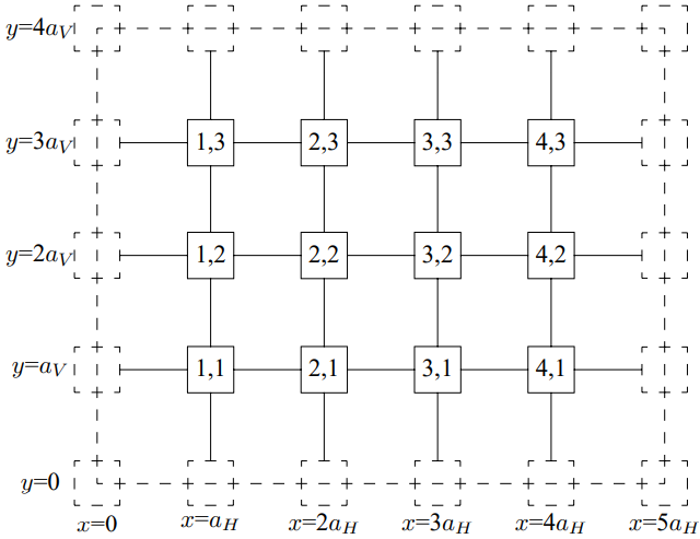
Figure \( 11.2\): A piece of an infinite two-dimensional beaded mesh.

The frequency of each mode is given by the dispersion relation (11.8): \[\omega^{2}=\frac{4 T_{H}}{m a_{H}} \sin ^{2} \frac{n \pi a_{H}}{2 L_{H}}+\frac{4 T_{V}}{m a_{V}} \sin ^{2} \frac{n^{\prime} \pi a_{V}}{2 L_{V}} .\]

These modes are animated in program 11-1.

The solution of this problem is an example of a technique called “separation of variables.” In the right variables, in this case, \(x\) and \(y\), the problem falls apart into one-dimensional problems. This trick works equally well in the continuous case, so long as the boundary surface is rectangular. If we take the limit in which \(a_{V}\) and \(a_{H}\) are very small compared to the wavelengths of interest, we can express (11.8) in terms of quantities that make sense in the continuum limit, just as in the analysis of the continuous one-dimensional string as the limit of the beaded string, in chapter 6. Assume, for simplicity, that \[a_{V}=a_{H}=a \text { and } T_{V}=T_{H}=T\]

(so that the \(x\) and \(y\) directions have the same properties). The quantities that characterize the surface in this case are the surface mass density, \[\rho_{s}=\frac{m}{a^{2}} ,\]

and the surface tension, \[T_{s}=\frac{T}{a} .\]

The surface tension is the pull per unit transverse distance exerted by the membrane. When these quantities remain finite as the separation, \(a\), goes to zero, (11.8) becomes \[\omega^{2}=\frac{T_{s}}{\rho_{s}}\left(k_{x}^{2}+k_{y}^{2}\right)=\frac{T_{s}}{\rho_{s}}|\vec{k}|^{2} .\]

An argument that is precisely analogous to that for the one-dimensional case shows that in this limit, \(\psi(x, y, t)\) satisfies the two-dimensional wave equation, \[\frac{\partial^{2}}{\partial t^{2}} \psi(x, y, t)=v^{2}\left(\frac{\partial^{2}}{\partial x^{2}}+\frac{\partial^{2}}{\partial y^{2}}\right) \psi(x, y, t)=v^{2} \vec{\nabla}^{2} \psi(x, y, t) .\]

Note that in this limit, the special properties of the \(x\) and \(y\) axes that were manifest in the finite system have completely disappeared from the equation of motion. The wave numbers \(k_{x}\) and \(k_{y}\) form a two-dimensional vector \(\vec{k}\). The infinite number of solutions to the dispersion relation (11.18) are just those obtained by rotating \(\vec{k}\) in all possible ways without changing its length. This makes it possible to solve for the normal modes in circular regions, for example. But we will not discuss these more complicated boundary conditions now. It is clear, however, that (11.13) is the solution for the rectangular region in the continuous case, and that the corresponding frequency is \[\omega^{2}=\frac{T_{s}}{\rho_{s}}\left[\left(\frac{n \pi}{L_{H}}\right)^{2}+\left(\frac{n^{\prime} \pi}{L_{V}}\right)^{2}\right] .\]

Now because the system is continuous, the integers \(n\) and \(n^{\prime}\) run from zero to infinity (though \(n=n^{\prime}\) is not interesting), or until the continuum approximation breaks down.

Three Dimensions

The beaded mesh cannot be extended to three dimensions because there is no transverse direction. But a system of masses connected by elastic rods can be three-dimensional, and indeed, this sort of system is a good model of an elastic solid. This system is rather complicated because each mass can move in all three directions. A two-dimensional version of this is illustrated in Figure \( 11.3\). This system is the same as Figure \( 11.1\) except that the strings have been replaced by light, elastic rods, so that system is in equilibrium even without the frame. Now we are interested in the oscillations of this system in the plane of the paper. Compared to Figure \( 11.1\), this system has twice as many degrees of freedom, because each block can move in both the \(x\) and \(y\) direction, while in Figure \( 11.1\), the blocks moved only

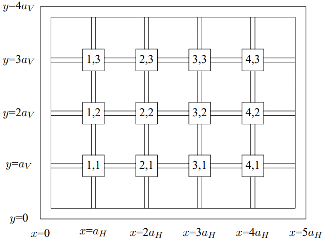
Figure \( 11.3\): A two-dimensional solid, with masses connected by elastic rods.

in the \(z\) direction. This means that we cannot use space translation invariance alone, even to determine the modes of the infinite system.

For each value of \(\vec{k}\), there will be four modes rather than the usual two. We would have to do some matrix analysis to see which combinations of \(x\) and \(y\) motion were actually the normal modes. We will not do this in general, but will discuss it briefly in the continuum limit, to remind you of some physics that is important for fields like geology.

Consider the continuous, infinite system obtained by taking the \(a\)’s very small in Figure \( 11.3\), with other quantities scaling appropriately. Consider a wave with wave number \(\vec{k}\). The normal modes will have the form \[\vec{A} e^{\pm \vec{k} \cdot \vec{r}} ,\]

for some vector \(\vec{A}\) (in the three-dimensional case, \(\vec{A}\) is a 3-vector, in our two-dimensional example, it is a 2-vector). If the system is rotation invariant, then there is no direction picked out by the physics except the direction of \(\vec{k}\). Then the normal modes must be a longitudinal or “compressional” mode \[\vec{A} \propto \vec{k} ,\]

and a transverse or “shear” mode \[\vec{A} \perp \vec{k} .\]

Each mode will have its own characteristic dispersion relation. In three dimensions, there will be two shear modes, because there are two perpendicular directions, and they will have the same dispersion relation, because one can be rotated into the other.

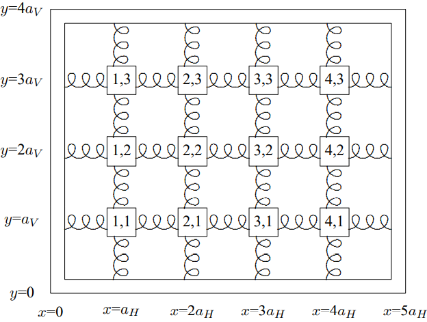
Figure \( 11.4\): A two-dimensional system of beads and springs.

Sound Waves

In a liquid or a gas, there are no shear waves because there is no restoring force that keeps the system in a particular shape. The shear modes have zero frequency. If we replaced the rods in Figure \( 11.3\) with unstretched springs, we would get a system with the same property, shown in Figure \( 11.4\). Without the frame, this system would not be rigid. However, the compressional modes are still there. These are analogous to sound waves. For an approximately continuous system like air, we expect a dispersion relation of the form \[\omega^{2}=v^{2} \vec{k}^{2}\]

where \(v\) is constant unless \(k\) is too large. We have already calculated \(v\), in (7.43), by considering one-dimensional oscillations. It is called the speed of sound because it is the speed of sound waves in an infinite or semi-infinite system.

We can describe the normal modes of a rectangular box full of air in terms of a function \(P(x, y, z)\) that describes the gas pressure at the point \((x, y, z)\). The pressure or density of the compressional wave is related to the displacement \(\vec{\psi}(x, y, z)\): \[\vec{\psi} \propto \vec{\nabla} P, \quad P \propto-\vec{\nabla} \cdot \vec{\psi} .\]

As in the two-dimensional system described above, we can use separation of variables and find a solution that is a product of functions of single variables. The only difference here is that the boundary conditions are different. Because of (11.25), which is the mathematical statement of the fact that gas is actually pushed from regions of high pressure to regions of low pressure, the pressure gradient perpendicular to the boundary must vanish. The gas at the boundary has nowhere to go. Thus the normal modes in a rectangular box, \(0 \leq x \leq X\), \(0 \leq y \leq Y\), \(0 \leq z \leq Z\), have the form \[P(x, y, z)=A \cos \left(n_{x} \pi x / X\right) \cos \left(n_{y} \pi y / Y\right) \cos \left(n_{z} \pi z / Z\right)\]

with frequency \[\omega^{2}=v^{2}\left(\left(\frac{n_{x} \pi}{X}\right)^{2}+\left(\frac{n_{y} \pi}{Y}\right)^{2}+\left(\frac{n_{z} \pi}{Z}\right)^{2}\right) .\]

The trivial solution \(n_{x} = n_{y} = n_{z} = 0\) represents stationary air. If any of the \(n^{\prime}\)s is nonzero, the mode is nontrivial.

___________________

¹There is a symmetry at work here! The modes in which the \(\vec{k}\) vector is lined up along the \(x\) or \(y\) axes are those that behave simply under reflections through the center of the rectangle.