11.3: Chladni Plates

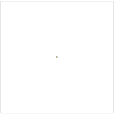
Figure \( 11.13\): A Chladni plate.

Chladni plates are a very pretty and instructive example of a two-dimensional oscillating system. A Chladni plate is simply a square metal plate that is driven transversely at its center. It is illustrated in Figure \( 11.13\). The dot in the center shows where the plate is driven in the transverse direction (out of the plane of the paper). The center, which we will take to have equilibrium position \(\vec{r} = 0\), moves up and down out of the plane of the paper at a frequency \(\omega\). Let us assume that the square sits in the \(x\)-\(y\) plane and has side \(2L\), and call the transverse displacement (in the \(z\) direction) \[\psi(x, y, t) \quad \text { for } \quad|x|,|y| \leq L .\]

In principle this is a forced oscillation problem. We could take the boundary condition at the origin to be \[\psi(0,0, t)=A \cos \omega t\]

and try to find \(\psi\) everywhere else.

To find \(\psi\), we must know the boundary condition at the edges of the plate. This depends on the details of the physics of the plate, because there are several ways that the plate can deform in response to the driving force. Just for simplicity, we will assume that the dominant deformation is shear, illustrated in Figure \( 11.14\). For this kind of displacement, to avoid an infinite acceleration, the slope of the plate must go to zero on the boundary in the direction perpendicular to the boundary, or in mathematics, \[\hat{n} \cdot \vec{\nabla} \psi=0\]

on the edge, where \(\hat{n}\) is a unit vector in the plane perpendicular to the edge. In this case, \[\left.\frac{\partial}{\partial x} \psi(x, y, t)\right|_{x=|L|}=\left.\frac{\partial}{\partial y} \psi(x, y, t)\right|_{y=|L|}=0 .\]

While the general case is more complicated than this, we will use (11.81) for illustration. The instructive thing about Chladni plates, as we will see, is not what is happening at the edges, but what is happening in the middle!

The general solution to this forced oscillation problem is not easy to write down. However, we are primarily interested in the resonances. Those are the modes of free oscillation of

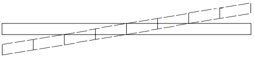
Figure \( 11.14\): Shear.

the plate (subject to the boundary condition (11.81)) that can be excited by the driving force. These will be those modes that have nonzero values of the displacement at the origin.

The relevant free oscillation modes of the plate have the form⁵ \[\psi_{\left(n_{x}, n_{y}\right)}(x, y, t)=A \cos \frac{n_{x} \pi x}{L} \cos \frac{n_{y} \pi y}{L} \cos \omega t\]

with \[\omega^{2}=\omega_{0}^{2}\left(\vec{k}^{2}\right) \Rightarrow \omega^{2}=f\left(n_{x}^{2}+n_{y}^{2}\right) .\]

If the frequencies of these modes were unique, (11.82) would be the whole story. But the interesting thing about this system is that the symmetry guarantees that there is degeneracy — that is that if \(n_{x} \neq n_{y}\), there are two modes with the same frequency. We can get a physically equivalent mode by interchanging \(n_{x} \longleftrightarrow n_{y}\), because this just corresponds to a \(90^{\circ}\) rotation of the plate, which doesn’t change the physics at all. When we have degenerate modes, then linear combinations of them are also modes, as shown in (3.117). Thus we have to ask which linear combinations are excited by the driving force? Another way of saying this is summarized in (11.83). Rotation invariance ensures that \(\omega^{2}\) depends only on \(n_{x}^{2}+n_{y}^{2}\).

In particular, it is clear that the difference \[\psi_{\left(n_{x}, n_{y}\right)}^{-}(x, y, t)=A\left(\cos \frac{n_{x} \pi x}{L} \cos \frac{n_{y} \pi y}{L}-\cos \frac{n_{y} \pi x}{L} \cos \frac{n_{x} \pi y}{L}\right) \cos \omega t\]

vanishes at the origin. Only the sum couples to the driving force! \[\psi_{\left(n_{x}, n_{y}\right)}^{+}(x, y, t)=A\left(\cos \frac{n_{x} \pi x}{L} \cos \frac{n_{y} \pi y}{L}+\cos \frac{n_{y} \pi x}{L} \cos \frac{n_{x} \pi y}{L}\right) \cos \omega t\]

These are the resonant modes of a Chladni plate.

One reason that this is amusing is that it is easy to see. If you excite the plate, and sprinkle sand on it, the sand builds up in the regions where the plate is not moving — along the displacement nodes where \(\psi=0\). Thus we can get a visual picture of the zeros of \(\psi\). Let’s look at some of these modes (in order of increasing frequency) to see what to expect.

The mode \(\psi_{(0,0)}^{+}\) is not interesting. It corresponds to the whole plate going up and down as a block. Obviously, the corresponding frequency is 0, because there is no restoring force. The first interesting mode is \[\psi_{(1,0)}^{+}(x, y, t)=A\left(\cos \frac{\pi x}{L}+\cos \frac{\pi y}{L}\right) \cos \omega t .\]

This vanishes for \[y=\pm L \pm x\]

so the Chladni sand pattern looks like the diagram in Figure \( 11.15\).

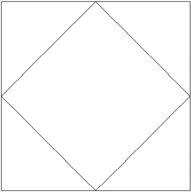
Figure \( 11.15\): The Chladni pattern for the mode \(\left(n_{x}, n_{y}\right)=(1,0)\).

The next mode is \[\psi_{(1,1)}^{+}(x, y, t)=2 A \cos \frac{\pi x}{L} \cos \frac{\pi y}{L} \cos \omega t .\]

Because this mode is not degenerate, it does not give rise to a very interesting pattern. It vanishes at \[x=\pm \frac{L}{2} \quad \text { or } \quad y=\pm \frac{L}{2} ,\]

which gives the pattern shown in Figure \( 11.16\). We won’t consider any more of these boring modes with \(n_{x} = n_{y}\).

The next mode is \[\psi_{(2,0)}^{+}(x, y, t)=A\left(\cos \frac{2 \pi x}{L}+\cos \frac{2 \pi y}{L}\right) \cos \omega t ,\]

which vanishes for \[y=\pm \frac{L}{2} \pm x \quad \text { or } \quad y=\pm \frac{3 L}{2} \pm x\]

so the pattern looks like Figure \( 11.17\).

Next comes \[\psi_{(2,1)}^{+}(x, y, t)=A\left(\cos \frac{\pi x}{L} \cos \frac{2 \pi y}{L}+\cos \frac{2 \pi x}{L} \cos \frac{\pi y}{L}\right) \cos \omega t .\]

This vanishes for \[\begin{gathered}
c_{x}\left(2 c_{y}^{2}-1\right)+c_{y}\left(2 c_{x}^{2}-1\right)=0 \\
=\left(c_{x}+c_{y}\right)\left(2 c_{x} c_{y}-1\right)=0
\end{gathered}\]

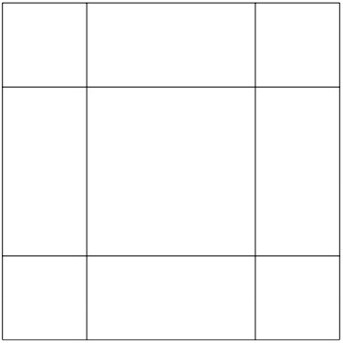
Figure \( 11.16\): The Chladni pattern for the mode (1,1).

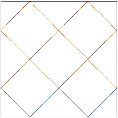
Figure \( 11.17\): The Chladni pattern for the mode (2,0).

with \(c_{x} \equiv \cos (\pi x / L)\) and \(c_{y} \equiv \cos (\pi y / L)\)9. The pattern is shown in figure 11.18.

We could go on, but you should have the idea by now. Let us look at one last mode: \[\psi_{(3,1)}^{+}(x, y, t)=A\left(\cos \frac{\pi x}{L} \cos \frac{3 \pi y}{L}+\cos \frac{3 \pi x}{L} \cos \frac{\pi y}{L}\right) \cos \omega t ,\]

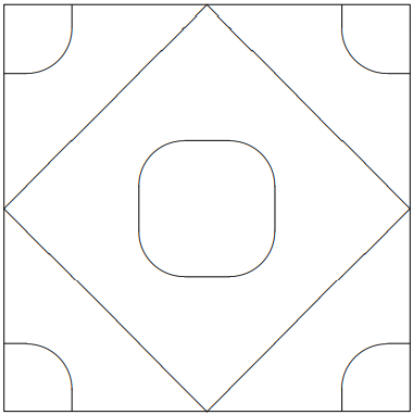
Figure \( 11.18\): The Chladni pattern for the mode (2,1).

vanishing for \[\begin{gathered}
c_{x}\left(4 c_{y}^{3}-3 c_{y}\right)+c_{y}\left(4 c_{x}^{3}-c_{x}\right)=0 \\
-c_{x} c_{y}\left(4 c_{x}^{2}+4 c_{y}^{2}-6\right)-0
\end{gathered}\]

with pattern shown in figure 11.19.

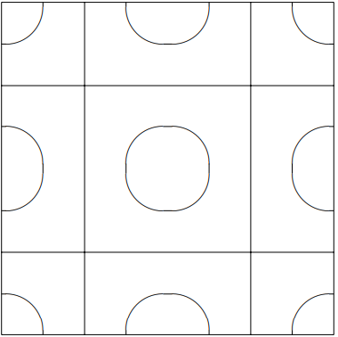
Figure \( 11.19\): The Chladni pattern for the mode (3,1).

Moral: When there is more than one mode with the same frequency, look at linear combinations to determine which are excited!

_________________

⁵There are also modes proportional to sin (nx + 1/2)πx/L and/or sin (ny + 1/2)πy/L, but these vanish at the origin and are not excited by the driving force.