11.2: Plane Boundaries

The easiest traveling waves to discuss in two and three dimensions are “plane waves,” solutions in the infinite system of the form \[\psi(r, t)=A e^{i(\vec{k} \cdot \vec{r}-\omega t)} .\]

This describes a wave traveling the direction of the wave-number vector, \(\vec{k}\), with the phase velocity in the medium. The displacement (or whatever) is constant on planes of constant \(\vec{k} \cdot \vec{r}\), which are perpendicular to the direction of motion, \(\vec{k}\). We will study more complicated traveling waves soon, when we discuss diffraction. Then we will learn how to describe “beams” of light or sound or other waves that are the traveling waves with which we usually work. We will see how to describe them as superpositions of plane waves. For now, you can think of a plane wave as being something like the traveling wave you would encounter inside a wide, coherent beam, or very far from a small source of nearly monochromatic light, light with a definite frequency. That should be enough to give you a physical picture of the phenomena we discuss in this section.

We are most interested in waves such as light and sound. However, it is much easier to discuss the transverse oscillations of a two-dimensional membrane, and many of our examples will be in that system. There are two reasons. One is that a two-dimensional membrane is easier to picture on two-dimensional paper. The other reason is that the physics is very simple, so we can concentrate on the wave properties. We will try to point out where things get more complicated for other sorts of wave phenomena.

Consider two two-dimensional membranes stretched in the \(z = 0\) plane, as shown in Figure \( 11.5\). For \(x < 0\), suppose that the surface mass density is \(\rho_{s}\) and surface tension \(T_{s}\). For \(x > 0\), suppose that the surface mass density is \(\rho_{s}^{\prime}\) and surface tension \(T_{s}^{\prime}\). This is a two-dimensional analog of the string system that we discussed at length in chapter 9. The boundary between the two membranes must supply a force (in this case, a constant force per unit length) in the \(x\) direction to support the difference between the tensions, as in the system of Figure \( 9.2\). However, we will assume that whatever the mechanism is that supplies this force, it is massless, frictionless and infinitely flexible.

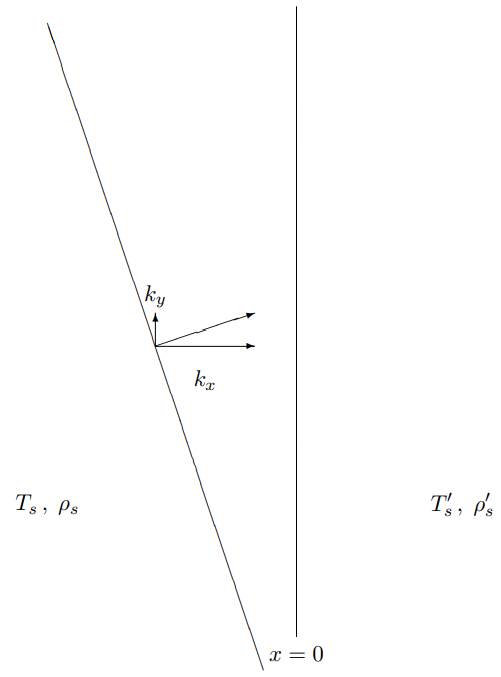
Figure \( 11.5\): A line of constant phase in a plane wave approaching a boundary.

Now again, we can consider reflection of traveling waves. Thus, suppose that there is, in this membrane, a plane wave with amplitude \(A\) and wave number \(\vec{k}\) for \(x < 0\), traveling in toward the boundary at \(x = 0\). The condition that the wave is traveling toward the boundary can be written in terms of the components of \(\vec{k}\) as \[k_{x}>0 .\]

We would like to know what waves are produced by this incoming wave because of reflection and transmission at the boundary, \(x = 0\). On general grounds of space translation invariance, we expect the solution to have the form \[\begin{aligned}
\psi(r, t)=A e^{i(\vec{k} \cdot \vec{r}-\omega t)}+\sum_{\alpha} R_{\alpha} A e^{i\left(\vec{k}_{\alpha} \cdot \vec{r}-\omega t\right)} & & \text { for } x \leq 0 \\
\psi(r, t)=\sum_{\beta} \tau_{\beta} A e^{i\left(\vec{k}_{\beta} \cdot \vec{r}-\omega t\right)} & & \text { for } x \geq 0
\end{aligned}\]

\[\vec{k}_{\alpha}^{2}=\omega^{2} \frac{\rho_{s}}{T_{s}} ; \quad \vec{k}_{\beta}^{2}=\omega^{2} \frac{\rho_{s}^{\prime}}{T_{s}^{\prime}} ,\]

and \[k_{\alpha x}<0 \text { and } k_{\beta_{x}}>0 \text { for all } \alpha \text { and } \beta .\]

The \(\alpha\) and \(\beta\) in (11.30) run over all the transmitted and reflected waves. We will show shortly that only one of each contributes for a plane boundary condition at \(x = 0\), but (11.30) is completely general, following just from space translation invariance. Note that we have put in boundary conditions at \(\pm \infty\) by requiring (11.29) and (11.32). Except for the incoming wave with amplitude \(A\), all the other waves are moving away from the boundary. But we have not yet put in the boundary condition at \(x = 0\).

Snell’s Law — the Translation Invariant Boundary

11-2
As far as we know from considerations of the physics at \(\pm \infty\), the reflected and transmitted waves could be a complicated superposition of an infinite number of plane waves going in various directions away from the boundary. In fact, if the boundary were irregularly shaped, that is exactly what we would expect. It is the fact that the boundary, \(x = 0\), is itself invariant under space translations in the \(y\) directions that allows us to cut down the infinite number of parameters in (11.30) to only two. Because translations in the \(y\) direction leave the whole system invariant, including the boundary, we can find solutions in which all the components have the same irreducible \(y\) dependence. If the incoming wave is proportional to \[e^{i k_{y} y} ,\]

then all the components of (11.30) must also be proportional to \(e^{i k_{y} y}\). Otherwise there is no way to satisfy the boundary condition at \(x = 0\) for all \(y\). That means that \[k_{\alpha y}=k_{y}, \quad k_{\beta_{y}}=k_{y} .\]

But (11.34), together with (11.31) and (11.32), completely determines the wave vectors \(\vec{k}_{\alpha}\) and \(\vec{k}_{\beta}\). Then (11.30) becomes² \[\begin{aligned}
\psi(r, t)=A e^{i \vec{k} \cdot \vec{r}-i \omega t}+R A e^{i \vec{k} \cdot \vec{r}-i \omega t} \equiv \psi_{-}(r, t) & & \text { for } x \leq 0 \\
\psi(r, t)=\tau A e^{i \vec{k}^{\prime} \cdot \vec{r}-i \omega t} \equiv \psi_{+}(r, t) & & \text { for } x \geq 0
\end{aligned}\]

where \[\tilde{k}_{y}=k_{y}, \quad k_{y}^{\prime}=k_{y} ,\]

and \[\tilde{k}_{x}=-\sqrt{\omega^{2} / v^{2}-k_{y}^{2}}=-k_{x}, \quad k_{x}^{\prime}=\sqrt{\omega^{2} / v^{\prime 2}-k_{y}^{2}} ,\]

with \[v=\sqrt{\frac{T_{s}}{\rho_{s}}}, \quad v^{\prime}=\sqrt{\frac{T_{s}^{\prime}}{\rho_{s}^{\prime}}} .\]

The entertaining thing about (11.35)-(11.37) is that we know everything about the directions of the reflected and transmitted waves, even though we have not even mentioned the details of the physics at the boundary. To get the directions, we needed only the invariance under translations in the \(y\) direction. The details of the physics of the boundary come in only when we want to calculate \(R\) and \(\tau\). The directions of the reflected and transmitted waves are the same for any system with a translation invariant boundary. Obviously, this argument works in three dimensions, as well. In fact, if we simply choose our coordinates so that the boundary is the \(x = 0\) plane and the wave is traveling in the \(x\)-\(y\) plane, then nothing depends on the \(z\) coordinate and the analysis is exactly the same as above. For example, we can apply these arguments directly to electromagnetic waves. For electromagnetic waves in a transparent medium, because the phase velocity is \(v_{\phi}=\omega / k\), the index of refraction,\(n\), is proportional to \(k\), \[n=\frac{c}{v_{\varphi}}=k \frac{c}{\omega} .\]

(11.36)-(11.37) shows that the reflected wave comes off at the same angle as the incoming wave because the only difference between the \(k\) vectors of the incoming and reflected waves is a change of the sign of the \(x\) component. Thus the angle of incidence equals the angle of reflection. This is the rule of “specular reflection.” From (11.36), we can also derive Snell’s law of refraction for the angle of the refracted wave. If \(\theta\) is the angle that the incident wave makes with the perpendicular to the boundary, and \(\theta^{\prime}\) is the corresponding angle for the transmitted wave, then (11.36) implies \[k \sin \theta=k^{\prime} \sin \theta^{\prime} .\]

For electromagnetic waves, we can rewrite this as \[n \sin \theta=n^{\prime} \sin \theta^{\prime} .\]

For example, when an electromagnetic wave in air encounters a flat glass surface at an angle \(\theta\), \(n^{\prime}>n\) in (11.41). The wave is refracted toward the perpendicular to the surface. This is illustrated in Figure \( 11.6\) for \(n^{\prime}>n\).

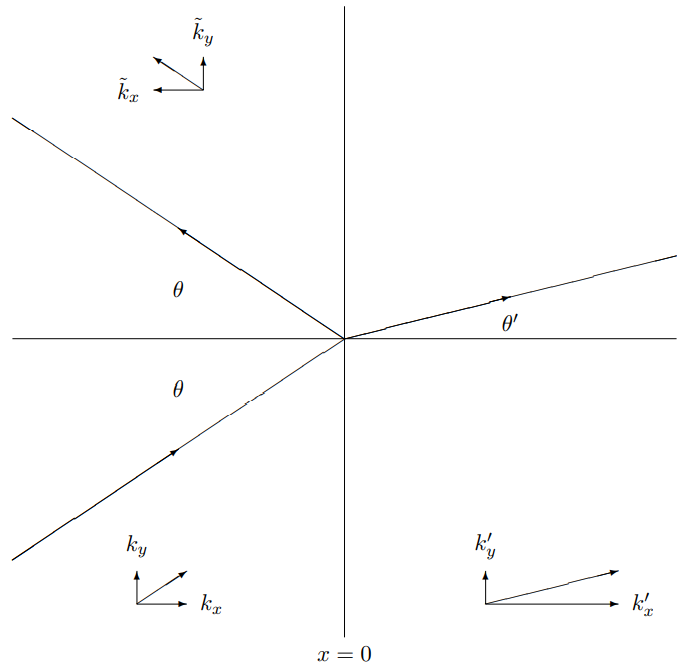
Figure \( 11.6\): Reflection and transmission from a boundary.

Let us now finish the solution for the membrane problem by solving for \(R\) and \(\tau\) in (11.35). To do this, we must finally discuss the boundary conditions in more detail. One is that the membrane is continuous, which from the form, (11.35), implies \[\left.\psi_{-}(r, t)\right|_{x=0}=\left.\psi_{+}(r, t)\right|_{x=0} ,\]

or \[1+R=\tau .\]

The other is that the vertical force on any small length of the membrane is zero. The force on a small length, \(d \ell\), of the boundary at the point, \((0, y, 0)\), from the membrane for \(x < 0\) is given by \[-\left.T_{s} d \ell \frac{\partial \psi_{-}(r, t)}{\partial x}\right|_{x=0} .\]

This is analogous to the one-dimensional example illustrated in Figure \( 8.6\). The force of surface tension is perpendicular to the boundary, so for small displacements, only the slope of the displacement in the \(x\) direction matters. The slope in the \(y\) direction gives no contribution to the vertical force to first order in the displacement. Likewise, the force on a small length, \(d \ell\), of the boundary at the point, \((0, y, 0)\), from the membrane for \(x > 0\) is given by \[\left.T_{s}^{\prime} d \ell \frac{\partial \psi_{+}(r, t)}{\partial x}\right|_{x=0} .\]

Thus the other boundary condition is \[\left.T_{s}^{\prime} d \ell \frac{\partial \psi_{+}(r, t)}{\partial x}\right|_{x=0}=\left.T_{s} d \ell \frac{\partial \psi_{-}(r, t)}{\partial x}\right|_{x=0} ,\]

or \[T_{s}^{\prime} k_{x}^{\prime} \tau=T_{s} k_{x}(1-R) .\]

Thus the solution is \[\tau=\frac{2}{1+r}, \quad R=\frac{1-r}{1+r},\]

where \[r=\frac{T_{s}^{\prime} k_{x}^{\prime}}{T_{s} k_{x}} .\]

You can see from (11.48) and (11.49) that we can adjust the surface tension to make the reflected wave go away even when there is a change in the length of the \(\vec{k}\) vector from one side of the boundary to the other. It is useful to think about refraction in this limit, because it will allow us to visualize it in a simple way. If \(r = 1\) in (11.48), then \(R = 0\) and \(\tau=1\). There is no reflected wave and the transmitted wave has the same amplitude as the incoming wave. Thus in each region, there is a single plane wave. Remember that a plane wave consists of infinite lines of constant phase perpendicular to the \(\vec{k}\) vector, moving in the direction of the \(k\) vector with the phase velocity, \(v_{\varphi}=\omega /|\vec{k}|\). In particular, suppose we look at lines on which the phase is zero, so that \(\psi=A\). The perpendicular distance between two such lines is the wavelength, \(2 \pi /|\vec{k}|\), because the phase difference between neighboring lines is \(2 \pi\). But here is the point. The lines in the two regions must meet at the boundary, \(x = 0\), to satisfy the boundary condition, (11.43). If the incoming wave amplitude is 1 at \(x = 0\), the outgoing wave amplitude is also 1. The lines where \(\psi=A\) are continuous across the boundary, \(x = 0\). This situation is illustrated in Figure \( 11.7\). The \(\vec{k}\) vectors in the two regions are shown. Notice that the angle of the lines must change when the distance between them changes in order to maintain continuity at the boundary. In program 11-2, the same system is shown in motion.

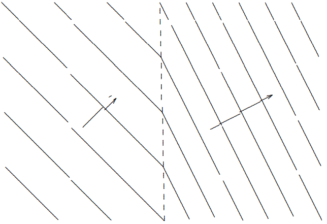
Figure \( 11.7\): Lines of constant \(\psi=1\) for a system with refraction but no reflection.

Prisms

The nontrivial index of refraction of glass is the building block of many optical elements. Let us discuss the prism. In fact, to do the problem of the scattering of light waves by prisms entirely correctly would require much more sophisticated techniques than we have at our disposal at the moment. The reason is that the prism is not an infinite, flat surface with space translation invariance. In general, we would have to worry about the boundary. However, we can say interesting things even if we ignore this complication. The idea is to think not of an infinite plane wave, but of a wide beam of light incident on a face of the prism. A wide beam behaves very much like a plane wave, and we will ignore the difference in this chapter. We will see what the differences are in Chapter 13 when we discuss diffraction.

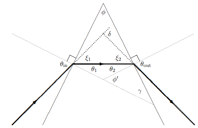
Figure \( 11.8\): The geometry of a prism.

Thus we consider the following situation, in which a wide beam of light enters one face of a prism with index of refraction \(n\) and exits the other face. The geometry is shown in Figure \( 11.8\) (the directions of the beams are indicated by the thick lines). The interesting quantity is \(\delta\). This describes how much the direction of the outgoing beam has been deflected from the direction of the incoming beam by the prism. We can calculate it using simple geometry and Snell’s law, (11.40). From Snell’s law \[\sin \theta_{\text {in }}=n \sin \theta_{1}\]

and \[\sin \theta_{\text {out }}=n \sin \theta_{2} .\]

Now for some geometry. \[\theta_{2}+\theta_{1}=\phi^{\prime}\]

— because the complement of \(\phi^{\prime}\), \(\pi-\phi^{\prime}\), along with \(\theta^{1}\) and \(\theta^{2}\) are the angles of a triangle, and thus add to \(\pi\). \[\phi=\phi^{\prime}\]

— because \(\phi\) and \(\phi^{\prime}\) are corresponding angles of the two similar right triangles with other acute angle \(\gamma\). Thus \[\delta=\xi_{1}+\xi_{2}=\theta_{\mathrm{in}}+\theta_{\mathrm{out}}-\theta_{1}-\theta_{2}=\theta_{\mathrm{in}}+\theta_{\mathrm{out}}-\phi\]

where we have used (11.52) and (11.53). But for small angles, from (11.50) and (11.51), \[\theta_{\mathrm{in}} \approx n \theta_{1}, \quad \theta_{\mathrm{out}} \approx n \theta_{2} .\]

Thus \[\delta \approx n\left(\theta_{1}+\theta_{2}\right)-\phi \approx(n-1) \phi .\]

The result, (11.56), is certainly reasonable. It must vanish when \(n \rightarrow 1\), because there is no boundary for \(n = 1\). If things are small and the answer is linear, it must be proportional to \(\phi\).

One of the most familiar characteristics of a prism results from the dependence of the index of refraction, \(n\), on frequency. This causes a beam of white light to break up into colors. For most materials, the index of refraction increases with frequency, so that blue light is deflected more than red light by the prism. The physics of the frequency dependence of \(n\) is that of forced oscillation. The index of refraction of a material is related to the dielectric constant (see (9.53)), that in turn is related to the distortion of the electronic structure of the material caused by the electric field. For a varying field, this depends on the amplitude of the motion of bound charges within the material in an electric field. Because these charges are bound, they respond to the oscillating fields in an electromagnetic wave like a mass on a spring subject to an oscillating force. We know from our studies of forced oscillation that this amplitude has the form \[\sum_{\underset{\alpha}{ }^{\text {resonances }}} \frac{C_{\alpha}}{\omega_{\alpha}^{2}-\omega^{2}} ,\]

where \(\omega_{\alpha}\) are the resonant frequencies of the system and the \(C_{\alpha}\) are constants depending on the details of how the force acts on the degrees of freedom. We can estimate the order of magnitude of these resonant frequencies with dimensional analysis, if we remember that any material consists of electrons and nuclei held together by electrical forces (and quantum mechanics, of course, but \(\hbar\) will not enter into our estimate except implicitly, in the typical atomic distance). The relevant quantities are³ \[\begin{aligned}
&\text { The charge of the proton } e \approx 1.6 \times 10^{-19} \mathrm{C}\\
&\text { The mass of the electron } m_{e} \approx 9.11 \times 10^{-31} \mathrm{~kg}\\
&\text { Typical atomic distance } \quad a \approx 10^{-10} \mathrm{~m}=1 \AA\\
&\text { The speed of light } \quad c=299,792,458 \mathrm{~m} / \mathrm{s}
\end{aligned}\]

In terms of these parameters, we would guess that the typical force inside the materials is of \(\frac{e^{2}}{4 \pi \epsilon 0 a^{2}}\) (from Coulomb’s law), and thus that the spring constant is of order \(\frac{e^{2}}{4 \pi \epsilon_{0} a^{3}}\) (the typical force over the typical distance). Thus we expect \[\omega_{\alpha}^{2} \approx \sqrt{\frac{e^{2}}{4 \pi \epsilon_{0} a^{3} m_{e}}}\]

and \[\lambda_{\alpha} \approx \frac{2 \pi c}{\omega_{\alpha}} \approx 2 \pi c \sqrt{\frac{4 \pi \epsilon_{0} a^{3} m_{e}}{e^{2}}} \approx 10^{-7} \mathrm{~m}=1000 \AA .\]

This is a wavelength in the ultraviolet region of the electromagnetic spectrum, shorter than that of visible light. That means that for visible light, \(\omega<\omega_{\alpha}\), and thus the displacement, (11.57), increases as \(\omega\) increases for visible light. The distortion of the electronic structure of the material caused by a varying electric field increases as the frequency increases in the visible spectrum. Thus the dielectric constant of the material increases with frequency. Thus blue light is deflected more.

Incidentally, this is the same reason that the sky is blue. Blue light is scattered more than red light because its frequency is closer to the important resonances of the air molecules.

Total Internal Reflection

The situation in which the wave comes from a region of large \(|\vec{k}|\) into a region of smaller \(|\vec{k}|\) has another feature that is surprising and very useful. This situation is depicted in Figure \( 11.9\) for a system with no reflection. For small, \(\theta\), as shown in Figure \( 11.9\), this looks rather

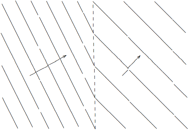
Figure \( 11.9\): Lines of constant \(\psi=1\) for \(n^{\prime} < n\).

like Figure \( 11.7\), except that the wave is refracted away from the perpendicular to the surface instead of toward it. But suppose that the angle \(\theta\) is large, satisfying \[n \sin \theta / n^{\prime}>1 .\]

Then there is no solution for real \(\theta^{\prime}\) in (11.41). Thus there can be no transmitted traveling wave. The incoming wave must be totally reflected by the boundary. This is total internal reflection. It happens when a plane wave tries to escape from a region of high \(|\vec{k}|\) to a region of lower \(|\vec{k}|\) at a grazing angle. It is extensively used in optical equipment and many other things. Let us investigate this peculiar phenomenon in more detail.

Suppose we start from \(\theta = 0\) and increase \(\theta\). As \(\theta\) increases, \(k_{y}\) increases and \(k_{x}\) decreases. This continues until we get to the boundary of total internal reflection, called the critical angle, \[\sin \theta=\sin \theta_{c} \equiv \frac{n^{\prime}}{n} .\]

The amplitudes for both the reflected and transmitted waves in (11.48) also increase. At the critical angle, \(k_{x}\) vanishes. The amplitude for the reflected wave is 1 and the amplitude for the transmitted wave is 2. However, even though the transmitted wave is nonzero, no energy is carried away from the boundary because the \(\vec{k}\) vector points in the \(y\) direction. As \(\theta\) increases beyond the critical angle, \(k_{y}\) continues to increase. To satisfy the dispersion relation, \[\omega^{2}=v^{\prime 2}\left(k_{x}^{2}+k_{y}^{2}\right) ,\]

\(k_{x}\) must be pure imaginary! The x dependence is then proportional to \[e^{-\kappa x} \text { where } \kappa=\operatorname{Im} k_{x} .\]

Now the nature of the boundary condition at infinity changes. We can no longer require simply that \(k_{x} > 0\). Instead, we must require \[\operatorname{Im} k_{x}>0 .\]

The sign is important. If \(\operatorname{Im} k_{x}\) were negative, the amplitude of the wave for \(x > 0\) would increase with \(x\), going exponentially to infinity as \(x \rightarrow \infty\). This doesn’t make much physical sense because it corresponds to a finite cause (the incoming wave for \(x < 0\)) producing an infinite effect. As we will see below, we can also come to this conclusion by going to this infinite system as a limit of a finite system.

We actually have three different boundary conditions at infinity for this situation: \[\begin{gathered}
\operatorname{Re} k_{x}>0 \text { for } \theta<\theta_{c} , \\
k_{x}=0 \text { for } \theta=\theta_{c} , \\
\operatorname{Im} k_{x}>0 \text { for } \theta>\theta_{c} .
\end{gathered}\]

These three can be combined into a compound condition that is valid in all regions: \[\operatorname{Re} k_{x} \geq 0, \quad \operatorname{Im} k_{x} \geq 0 .\]

The condition, (11.67), is actually the most general statement of the outgoing traveling wave boundary condition at infinity. It is also correct in situations in which there is damping and both the real and imaginary parts of \(k_{x}\) are nonzero. This is the mathematical statement of the physical fact that the wave for \(x > 0\), whatever its form, is produced at the boundary by the incoming wave.

From (11.48) and (11.49), you see that for \(\theta>\theta_{c}\), the amplitude of the reflected wave becomes complex. However, its absolute value is still 1. All the energy of the incoming wave is reflected.

We have seen that in total internal reflections, the wave does penetrate into the forbidden region, but the \(x\) dependence is in the form of an exponential standing wave, not a traveling wave. The \(y\) dependence is that of a traveling wave. This is one of many situations in which the physics forces the nature of the two- or three-dimensional solution to have different properties in different directions.

It is easy to see total internal reflection in a fish-tank, a glass block, or some other rectangular transparent object with an index of refraction significantly greater than 1. You can look through one face of the rectangle and see the silvery reflection from an adjacent face, as illustrated in Figure \( 11.10\).

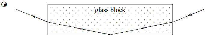
Figure \( 11.10\): Total internal reflection in glass with index of refraction 2.

Tunneling

Consider the scattering of a plane wave in the system illustrated in Figure \( 11.11\). This is the same setup as in Figure \( 11.10\), except that another block of glass has been added a small distance, \(d\), below the boundary from which there was total internal reflection. We have defined the positive \(x\) direction to be downwards for consistency with the discussion of Snell’s law, above. Now does any of the light get through to the observer below, or is the light still totally reflected at the boundary, as in Figure \( 11.10\)? The answer is that some light gets through. As we will see in detail in an example below, the presence of the other block of glass means that instead of a boundary condition at infinity, we have a boundary condition at the finite distance, \(d\).

The details of this phenomenon for electromagnetic waves are somewhat complicated by polarization, which we will discuss in detail in the next chapter. However, there is a precisely analogous process in the transverse oscillation of membranes that we can analyze easily

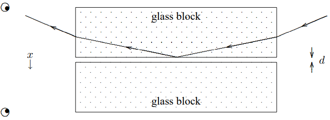
Figure \( 11.11\): A simple experiment to demonstrate tunneling.

In fact, we will find that we have already analyzed it in chapter 9. Consider the scattering problem illustrated in Figure \( 11.12\). The unshaded region is a membrane with lower density. The arrows indicate the directions of the \(\vec{k}\) vectors of the plane waves. The shaded regions

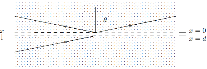
Figure \( 11.12\): Tunneling in an infinite membrane.

have surface mass density \(\rho_{s}\) and surface tension \(T_{s}\). The unshaded region, which extends from \(x = 0\) to \(x = d\), has the same surface tension but surface mass density \(\rho_{s} / 4\). Thus the ratio of phase velocities in the two regions is two, the same as the ratio from air to glass in Figure \( 11.11\). The dashed lines are massless boundaries between the different membranes.

We can now ask what are the coefficients, \(R\) and \(\tau\), for reflection and transmission. We have done this problem for a single boundary earlier in this chapter in (11.42)-(11.49). We could solve this one by putting two of these solutions together using the transfer matrix techniques of chapter 9. In fact, we do not even have to do that, because we can read off the result from (9.97) and (9.98) in the discussion of thin films in chapter 9. The point is that all the terms in our solution must have the same irreducible \(y\) dependence, \(e^{i k_{y} y}\), because of the space translation invariance of the whole system including the boundary in the \(y\) direction. This common factor plays no role in the boundary conditions. If we factor it out, what is left looks like a one-dimensional scattering problem. Comparing (11.47) for \(T_{s}=T_{s}^{\prime}\) (9.10), you can see that the analyses become the same if we make the replacements \[\begin{aligned}
k_{1} & \rightarrow k_{x} \\
k_{2} & \rightarrow k_{x}^{\prime} \\
L & \rightarrow d
\end{aligned}\]

where \(k_{x}\) is the \(x\) component of the \(\vec{k}\) vector of the incoming wave in the shaded region and \(k_{x}^{\prime}\) is the \(x\) component of the \(\vec{k}\) vector of the transmitted wave in the unshaded region. The result is \[\tau=\left(\cos k_{x}^{\prime} d-i \frac{k_{x}^{2}+k_{x}^{\prime 2}}{2 k_{x} k_{x}^{\prime}} \sin k_{x}^{\prime} d\right)^{-1} e^{-i k_{x} d}\]

and \[R=\left(i \frac{k_{x}^{2}-k_{x}^{\prime 2}}{2 k_{x} k_{x}^{\prime}} \sin k_{x}^{\prime} d\right)\left(\cos k_{x}^{\prime} d-i \frac{k_{x}^{2}+k_{x}^{\prime 2}}{2 k_{x} k_{x}^{\prime}} \sin k_{x}^{\prime} d\right)^{-1} .\]

It may be a little easier to look at the intensity of the transmitted wave, which is proportional to \[|\tau|^{2}=\frac{2 k_{x}^{2} k_{x}^{2}}{\left(k_{x}^{4}+k_{x}^{\prime 4}\right) \sin ^{2} k_{x}^{\prime} d+2 k_{x}^{2} k_{x}^{\prime 2}} .\]

Note that we have not mentioned the critical angle or total internal reflection or anything like that. The reason is that our analysis in chapter 9 was perfectly general. It remains correct even if the angular wave number in the middle region becomes imaginary. All that happens for \(\theta\) larger than the critical angle, \(\theta_{c}\), is that \(k_{x}^{\prime}\) becomes imaginary. But this has a spectacular effect in (11.71). If \(k_{x}^{\prime} \rightarrow i \kappa\), where \(\kappa\) is real, then it follows from the Euler identity, (1.57) x and (1.62), that \[\sin k_{x}^{\prime} d \rightarrow i \sinh \kappa d ,\]

where \(\sinh\) is the “hyperbolic sine”, defined by \[\sinh x \equiv \frac{e^{x}-e^{-x}}{2} .\]

Thus for angles above the critical angle, the denominator of (11.71) is an exponentially increasing function of \(d\) (the \(e^{\kappa d}\) term in (11.73) dominates for large \(\kappa d\)). The intensity of the transmitted wave therefore decreases exponentially with \(d\). In the limit of large \(d\), we quickly recover total internal reflection.

We can get some insight about what is happening by looking at the boundary conditions at \(x = d\) for angles above the critical angle. For \(x > d\), the wave has the form (suppressing the common factors of \(e^{i k_{y} y}\) and \(A e^{-i \omega t}\)) \[\tau e^{i k_{x} x} .\]

For \(0 \leq x \leq d\), the wave has the form \[T_{I I} e^{-\kappa x}+R_{I I} e^{\kappa x} ,\]

where I have called the coefficients \(T_{I I}\) and \(R_{I I}\) by analogy with transmitted and reflected waves, even though these are not traveling waves. The boundary conditions at \(x = d\) are \[\begin{gathered}
\tau e^{i k_{x} d}=T_{I I} e^{-\kappa d}+R_{I I} e^{\kappa d} , \\
i k_{x} \tau e^{i k_{x} d}=\kappa\left(-T_{I I} e^{-\kappa d}+R_{I I} e^{\kappa d}\right) .
\end{gathered}\]

This looks more complicated than it really is. If we solve for \(T_{I I} e^{-\kappa d}\) and \(R_{I I} e^{\kappa d}\) in terms of \(\tau e^{i k_{x} d}\), the result is \[T_{I I} c^{-\kappa d}=\frac{2 \kappa}{\kappa-i k_{x}} \tau c^{i k_{x} d}, \quad R_{I I} e^{\kappa d}=\frac{2 \kappa}{\kappa+i k_{x}} \tau c^{i k_{x} d} .\]

The important point is that the values of the two components of the wave, (11.75), at \(x = d\), \(T_{I I} e^{-\kappa d}\) and \(R_{I I} e^{-\kappa d}\), are more or less the same size. These two quantities do not have any exponential dependence on \(d\). This qualitative fact does not depend on the details of (11.76). It will be true for any reasonable boundary condition at \(x = d\).

Thus the coefficient, \(R_{I I}\) of the “reflected” wave (in quotes because it is a real exponential wave, not a traveling wave) must be smaller than the “transmitted” wave by a factor of roughly \(e^{2 \kappa d}\). Notice that this justifies the statement, (11.67), of the boundary condition at infinity. As \(d \rightarrow \infty\), for any reasonable physics at \(d\), the wave becomes a pure negative exponential.

At \(x = 0\), for large \(\kappa d\), the \(R_{I I}\) term in wave will be completely negligible, and \(T_{I I}\) term will be produced with some coefficient of order 1, just as in the limit of total internal reflection.

Thus what is happening in the boundary conditions for tunneling can be described qualitatively as follows. The incoming wave for \(x < 0\) produces the \(e^{-\kappa x}\) term in the region \(0 \leq x \leq d\), with an exponentially small admixture of \(e^{\kappa x}\). But at \(x = d\), the two parts of the exponential wave are of the same size (both exponentially small), and they can produce the transmitted wave.

The rapid exponential dependence of the transmitted wave on \(d\) has some interesting consequences. It implies, for example, that the reflected wave is also very sensitive to the value of \(d\), for small \(d\) (energy conservation implies \(|R|^{2}+|\tau|^{2}=1\)). You can see this rapid dependence in the example of (11.10) by putting your finger on the bottom surface of the glass block or fish tank, where the wave is being reflected. You will see a ghostly fingerprint! The reason is that the tiny indentations on your finger are far enough away from the glass that \(\kappa d\) is large and the wave is almost entirely reflected. But where the flesh is pressed tightly against the glass, the wave is absorbed. This is a simple version of a tunneling microscope.

Finally, before leaving the subject of tunneling, let us consider what happens when we turn down the intensity of the light wave in Figure \( 11.11\) so that we see the scattering of individual photons. The first thing to note is that each photon is either transmitted or reflected. The meaning of \(R\) and \(\tau\) in this case is that the \(|R|^{2}\) and \(|\tau|^{2}\) are the probabilities of reflection and transmission. You cannot predict whether any particular photon will get through. In the quantum mechanical world, you can predict only the probabilities.

The second thing to note is that in the particle description, the whole phenomenon of tunneling is very peculiar. A classical photon, coming at the boundary of the glass plate at more than the critical angle could not enter at all into the air. It would be forbidden to do so by conservation of energy and conservation of the \(y\) component of momentum.⁴ How can the particle get through to the \(x > d\) side if it cannot exist for \(0 < x < d\)? Obviously, in classical physics, it cannot. Tunneling is, therefore, a truly quantum mechanical phenomenon. The wave manages to penetrate into the forbidden region, but only in the form of a real exponential wave, not a traveling wave. It is only for \(x < 0\) and \(x > d\), where the waves are traveling, that they can be interpreted as particles in anything like the classical sense.

__________________

²We have defined \(\psi_{\pm}\) here to make it easier to discuss the boundary conditions, below.
³Note that it is the mass of the electron rather than the mass of the proton that is relevant, because the electrons move much more in electric fields.
⁴The boundary does not change \(p_{y}\) of the photon, because of the translation invariance in the \(y\) direction. However, there is no reason why the boundary cannot exert a force in the \(x\) direction and change \(p_{x}\) of the photon.