4.4: Conductors in Electrostatic Equilibrium

Learning Objectives

• List the six properties of a conductor in electrostatic equilibrium.
• Explain why no electric field may exist inside a conductor in electrostatic equilibrium.
• Explain why electric potential is constant throughout a conductor in electrostatic equilibrium.
• Explain how surface curvature affects surface charge and electric field in a conductor in electrostatic equilibrium.
• Describe the electric field and surface charge density in an empty cavity in a conductor in electrostatic equilibrium.

Recall that when a conductor is in electrostatic equilibrium, all the charges are stationary. Conductors in electrostatic equilibrium have several interesting properties:

Property \(\PageIndex{1}\): Electric Field Inside Conductors

The electric field is zero inside a conductor.

Proof: Suppose that there was a nonzero electric field inside the conductor. We know then that an electric force would be exerted on the charge. This force would cause the charges to accelerate. However, moving charges violate the assumption that the conductor is in electrostatic equilibrium. Thus, the electric field \(\vec{E}_{in}=0\) inside the conductor must be zero.

Property \(\PageIndex{2}\): Electric Potential Inside Conductors

The electric potential is a constant everywhere inside and on the surface of the conductor.

Proof: Consider a path in the conductor between any two Points A and B. From Electric Potential from Electric Field, we know that the change of potential between the points is given by

\[ \Delta V_{BA} = V_B-V_A =\int_A^B \vec{E}_{in} \cdot d\vec{l} = \int_A^B 0 \cdot d\vec{l} = 0 . \nonumber \]

Hence \(V_B - V-A = 0\) or \(V_B = V_A \). But because the choice of Points A and B were arbitrary, it must be that the potential is everywhere the same throughout the conductor, and the surface of the conductor must also be an equipotential. (Note: This statement does not claim that the potential must be zero; it can be any constant value.)

Property \(\PageIndex{3}\): Electric Field on Surface of Conductors

The exterior electric field is perpendicular to the surface of the conductor, beginning or ending on charges on the surface.

Proof: Because the surface is an equipotential, it follows that

\[ \Delta V_{BA} = V_B-V_A =\int_A^B \vec{E}_{in} \cdot d\vec{l} = 0 . \nonumber \]

The only way the integral can always be zero is if \( \vec{E}_{in} \cdot d\vec{l} = |\vec{E}||d\vec{l}|\cos\theta = 0 \). However, this relationship can only hold in general if \(\theta=0\). In other words, the electric field must be everywhere perpendicular to the displacements along the surface of the conductor (Fig. \(\PageIndex{1}\). (Alternatively, if the electric field were not perpendicular, then there would be force on the charge on the surface that would cause it to accelerate, thereby violating the assumption of electrostatic equilibrium.)

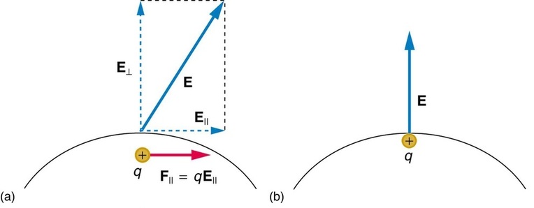
Figure \(\PageIndex{1}\): When an electric field \(\vec{E}=\mathbf{E}\) is applied to a conductor, free charges inside the conductor move until the field is perpendicular to the surface. (a) The electric field is a vector quantity, with both parallel and perpendicular components. The parallel component (\(\vec{E}_{||}=\mathbf{E}_{||}\)) exerts a force (\(\vec{F}_{||}=\mathbf{F}_{||}\)) on the free charge \(q\), which moves the charge until \(\vec{F}=\mathbf{F}=0\). (b) The resulting field is perpendicular to the surface. The free charge has been brought to the conductor’s surface, leaving electrostatic forces in equilibrium. [Image from OpenStax College Physics Figure 18.26].

Property \(\PageIndex{4}\): Excess Charge on Conductors

Any free excess charge resides entirely on the surface or surfaces of a conductor.

Plausibility Argument: Because all the excess charges are free to move in the conductor, they will repel each other as much as possible. Having the charge on the surface will achieve this result. (A mathematical proof is provided in the section Conductors in Electrostatic Equilibrium via Gauss's Law.)

Remarkably all of these properties will hold true simultaneously for any conductor regardless of its shape. As an example, Fig. \(\PageIndex{2}\) shows the result of placing a neutral conductor in an originally uniform electric field. The field becomes stronger near the conductor but entirely disappears inside it.

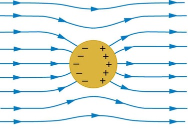
Figure \(\PageIndex{2}\): This illustration shows a spherical conductor in static equilibrium with an originally uniform electric field. Free charges move within the conductor, polarizing it, until the electric field lines are perpendicular to the surface. The field lines end on excess negative charge on one section of the surface and begin again on excess positive charge on the opposite side. No electric field exists inside the conductor, since free charges in the conductor would continue moving in response to any field until it was neutralized.

Charged Parallel Plates

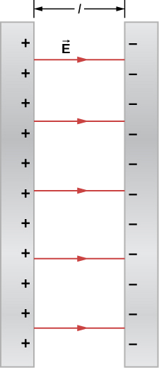
One of the most important cases of conductors in electrostatic equilibrium is the familiar parallel conducting plates shown in Figure \(\PageIndex{3}\). Between the plates, the equipotentials are evenly spaced and parallel. The same field could be maintained by placing conducting plates at the equipotential lines at the potentials shown.

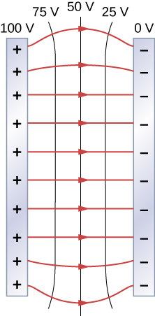
Figure \(\PageIndex{3}\): The electric field and equipotential lines between two metal plates. Note that the electric field is perpendicular to the equipotentials and hence normal to the plates at their surface as well as in the center of the region between them.

Based on what we know about electric potenial and electric field, we can also solve some quantitative problems about equipotentials, as shown in Examples \(\PageIndex{1}\) and \(\PageIndex{2}\).

Example \(\PageIndex{1}\): Calculating Equipotential Lines

You have seen the equipotential lines of a point charge in Figure \(\PageIndex{1}\). How do we calculate them? For example, if we have a \(+10\text{-nC}\) charge at the origin, what are the equipotential surfaces at which the potential is (a) 100 V, (b) 50 V, (c) 20 V, and (d) 10 V?

Strategy

Set the equation for the potential of a point charge equal to a constant and solve for the remaining variable(s). Then calculate values as needed.

Solution

In \(V = k\dfrac{q}{r}\), let \(V\) be a constant. The only remaining variable is \(r\); hence, \(r = k\dfrac{q}{V} = \text{constant}\). Thus, the equipotential surfaces are spheres about the origin. Their locations are:

1. \(r = k\dfrac{q}{V} = \left(8.99 \times 10^9 \, \mathrm{N}\cdot\mathrm{m}^2/\mathrm{C}^2\right) \dfrac{(10 \times 10^{-9}\,\mathrm{C})}{100 \,\mathrm{V}} = 0.90 \,\mathrm{m}\);
2. \(r = k\dfrac{q}{V} = \left(8.99 \times 10^9 \, \mathrm{N}\cdot\mathrm{m}^2/\mathrm{C}^2\right) \dfrac{(10 \times 10^{-9}\,\mathrm{C})}{50 \,\mathrm{V}} = 1.8 \, \mathrm{m}\);
3. \(r = k\dfrac{q}{V} = \left(8.99 \times 10^9 \, \mathrm{N}\cdot\mathrm{m}^2/\mathrm{C}^2\right) \dfrac{(10 \times 10^{-9}\,\mathrm{C})}{20 \,\mathrm{V}} = 4.5 \,\mathrm{m}\);
4. \(r = k\dfrac{q}{V} = \left(8.99 \times 10^9 \, \mathrm{N}\cdot\mathrm{m}^2/\mathrm{C}^2\right) \dfrac{(10 \times 10^{-9}\,\mathrm{C})}{10 \,\mathrm{V}} = 9.0 \,\mathrm{m}\).

Significance

This means that equipotential surfaces around a point charge are spheres of constant radius, as shown earlier, with well-defined locations.

Example \(\PageIndex{2}\):Potential Difference betwwen Oppositely Charged Parallel Plates

Two large conducting plates carry equal and opposite charges, with a surface charge density \(\sigma\) of magnitude \(6.81 \times 10^{-7}\, \mathrm{C}/\mathrm{m}\), as shown in Figure \(\PageIndex{4}\). The separation between the plates is \(l = 6.50 \,\mathrm{mm}\).

1. What is the electric field between the plates?
2. What is the potential difference between the plates?
3. What is the distance between equipotential planes which differ by 100 V?

Figure \(\PageIndex{4}\): The electric field between oppositely charged parallel plates. A portion is released at the positive plate.

Strategy

1. Since the plates are described as “large” and the distance between them is not, we will approximate each of them as an infinite plane.
2. Use \(\Delta V_{AB} = - \int_A^B \vec{E} \cdot d\vec{l}\).
3. Since the electric field is constant, find the ratio of 100 V to the total potential difference; then calculate this fraction of the distance.

Solution

a. The electric field is directed from the positive to the negative plate as shown in the figure, and its magnitude is given by (Common Models of Electric Potential)

\[ \begin{align*} E &= \dfrac{\sigma}{\epsilon_0} \\[4pt] &= \dfrac{6.81 \times 10^{-7}\,\mathrm{C}/\mathrm{m}^2}{8.85 \times 10^{-12}\,\mathrm{C}^2/\mathrm{N} \cdot \mathrm{m}^2} \\[4pt] &= 7.69 \times 10^4 \,\mathrm{V}/\mathrm{m}. \end{align*} \]

b. To find the potential difference \(\Delta V\) between the plates, we use a path from the negative to the positive plate that is directed against the field. The displacement vector \(d\vec{l}\) and the electric field \(\vec{E}\) are antiparallel so \(\vec{E} \cdot d\vec{l} = - E \, dl\). The potential difference between the positive plate and the negative plate is then

\[ \begin{align*} \Delta V &= - \int E \cdot dl \\[4pt] &= E \int dl \\[4pt] &= El \\[4pt] &= (7.69 \times 10^4\,\mathrm{V}/\mathrm{m})(6.50 \times 10^{-3}\,\mathrm{m}) \\[4pt] &= 500 \,\mathrm{V} \end{align*} \]

c. The total potential difference is 500 V, so 1/5 of the distance between the plates will be the distance between 100-V potential differences. The distance between the plates is 6.5 mm, so there will be 1.3 mm between 100-V potential differences.

Significance

You have now seen a numerical calculation of the locations of equipotentials between two charged parallel plates.

Exercise \(\PageIndex{1}\)

What are the equipotential surfaces for an infinite line charge?

Answer

infinite cylinders of constant radius, with the line charge as the axis

Falstad Simulation: 3D Electrostatic Field Simulation

Explore the 3-D Electrostatic Field Simulation (Java applet from Falstad.com). Start your investigation with a pair of parallel plates of equal but opposite charge.

Instructions:

1. Set the field selection to "charged plate pair."
2. Set the slice to "Show Y Slice."
3. Set the display to "Field Vectors." Describe the electric field-vector diagram. (Is it is similar to the diagram in Fig. \(\PageIndex{6}\)?)
4. Set the display to "Field Lines." Is the field-line diagram consistent with the field-vector diagram?
5. Set the display to "Equipotentials." Are the equipotentials consistent with the field vectors?
6. Vary the sheet size and sheet separation. Can you create a uniform field between the plates?

Next, explore other geometries we have discussed (finite line, charged line, charged ring, conducting plate) and investigate their electric field and equipotential diagrams.

Distribution of Charges on Curved Conductors

In Example \(\PageIndex{1}\) with a point charge, we found that the equipotential surfaces were in the form of spheres, with the point charge at the center. Given that a conducting sphere in electrostatic equilibrium is a spherical equipotential surface, we should expect that we could replace one of the surfaces in Example \(\PageIndex{2}\) with a conducting sphere and have an identical solution outside the sphere. We also know that the electric field must be zero inside the conductor. The electric field of the sphere may therefore be written as

\[\begin{array}{ccll}
E & = & 0 & (r < R), \\
E & = & \dfrac{1}{4 \pi \epsilon_0} \dfrac{q}{r^2} \hat{r} & (r \geq R).
\end{array}\]

To find the electric potential inside and outside the sphere, note that for \(r \geq R\), the potential must then be the same as that of an isolated point charge \(q\) located at \(r = 0\),

\[V(r) = \dfrac{1}{4\pi \epsilon_0} \dfrac{q}{r}, (r \geq R)\]

simply due to the similarity of the electric field.

For \(r < R, \, E = 0\), so \(V(r)\) is constant in this region. Since \(V(R) = q/4\pi \epsilon_0 R\),

\[V(r) = \dfrac{1}{4 \pi \epsilon_0} \dfrac{q}{R} (r < R).\]

With this background, we can now state an additional property of a conductor at electrostatic equilibrium.

Property \(\PageIndex{5}\): Surface Charge Density on Conductors

The surface charge density is inversely proportional to the local radius of curvature on the surface of a conductor.

Proof: Our goal will be to show that

\[\dfrac{\sigma_1}{\sigma_2} = \dfrac{R_2}{R_1}, \nonumber \]

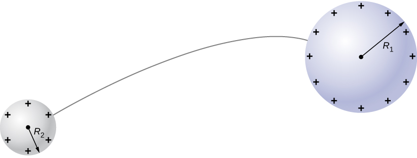
for two conducting spheres of radii \(R_1\) and \(R_2\), with surface charge densities \(\sigma_1\) and \(\sigma_2\) respectively, that are connected by a thin wire, as shown in Figure \(\PageIndex{5}\). The spheres are sufficiently separated so that each can be treated as if it were isolated (aside from the wire). Note that the connection by the wire means that this entire system must be an equipotential.

Figure \(\PageIndex{5}\): Two conducting spheres are connected by a thin conducting wire.

We have just seen that the electrical potential at the surface of an isolated, charged conducting sphere of radius \(R\) is

\[V = \dfrac{1}{4\pi \epsilon_0} \dfrac{q}{R}. \nonumber\]

Now, the spheres are connected by a conductor and are therefore at the same potential; hence

\[\dfrac{1}{4\pi \epsilon_0} \dfrac{q_1}{R_1} = \dfrac{1}{4\pi r\epsilon_0} \dfrac{q_2}{R_2}, \nonumber \] and

\[\dfrac{q_1}{R_1} = \dfrac{q_2}{R_2}. \nonumber \]

The net charge on a conducting sphere and its surface charge density are related by \(q = \sigma (4\pi R^2)\). Substituting this equation into the previous one, we find

\[\sigma_1 R_1 = \sigma_2 R_2. \nonumber \]

from which it follows that

\[\dfrac{\sigma_1}{\sigma_2} = \dfrac{R_2}{R_1}, \nonumber \]

showing that the surface charge density is inversely proportional to the radius of curvature of the sphere.

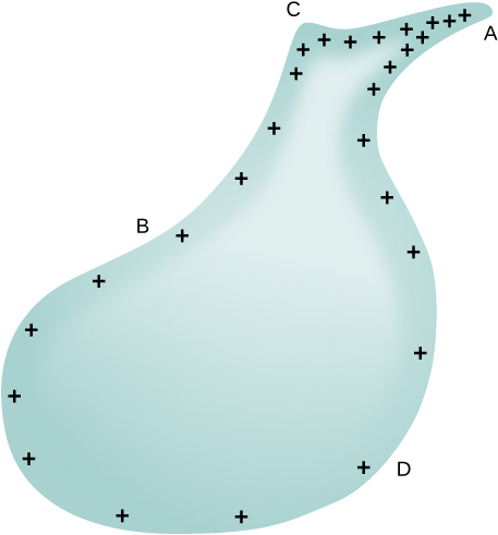
Obviously, two spheres connected by a thin wire do not constitute a typical conductor with a variable radius of curvature, but this result still holds true even in the more general case. The equation indicates that where the radius of curvature is large (points \(B\) and \(D\) in \(\PageIndex{10}\)), \(\sigma\) and \(E\) are small. Similarly, the charges tend to be denser where the curvature of the surface is greater, as demonstrated by the charge distribution on oddly shaped metal (Figure \(\PageIndex{6}\)). The surface charge density is higher at locations with a small radius of curvature than at locations with a large radius of curvature.

Figure \(\PageIndex{6}\): The surface charge density and the electric field of a conductor are greater at regions with smaller radii of curvature.

Electric Fields on Curved Surfaces

Having established that the surface charge density varies on the surface of a charged object based on the local curvature of the surface, one might expect that the electric field magnitude will also vary, and this is indeed true.

Property \(\PageIndex{6}\): Electric Field Magnitude on the Surface of a Conductor

The electric field magnitude on the curved surface of a conductor is inversely proportional to the radius curvature of the surface.

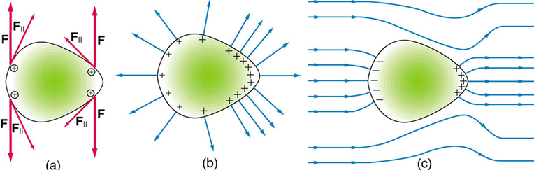
To see how and why this happens, consider the charged conductor in Fig. \(\PageIndex{7}\). Qualitatively, the electrostatic repulsion of like charges is most effective in moving them apart on the flattest surface, and so they become least concentrated there. This is because the forces between identical pairs of charges at either end of the conductor are identical, but the components of the forces parallel to the surfaces are different. The component parallel to the surface is greatest on the flattest surface and, hence, more effective in moving the charge (Fig. \(\PageIndex{7}a\)). The result is that the electric field is higher at sharper corners (Fig. \(\PageIndex{7}b\)). In fact, it is possible to show that the local electric field \(E = \sigma / \epsilon_0\) (see Conductors in Electrostatic Equilibrium Via Gauss's Law).

The same effect is produced on a conductor by an externally applied electric field (\(\PageIndex{7}c\)). Since the field lines must be perpendicular to the surface, more of them are concentrated on the most curved parts.

Figure \(\PageIndex{7}\): Excess charge on a nonuniform conductor becomes most concentrated at the location of greatest curvature. (a) The forces between identical pairs of charges at either end of the conductor are identical, but the components of the forces parallel to the surface are different. It is \(\vec{F}_{||}\) that moves the charges apart once they have reached the surface. (b) \(\vec{F}_{||}\) is smallest at the more pointed end, the charges are left closer together, producing the electric field shown. (c) An uncharged conductor in an originally uniform electric field is polarized, with the most concentrated charge at its most pointed end.

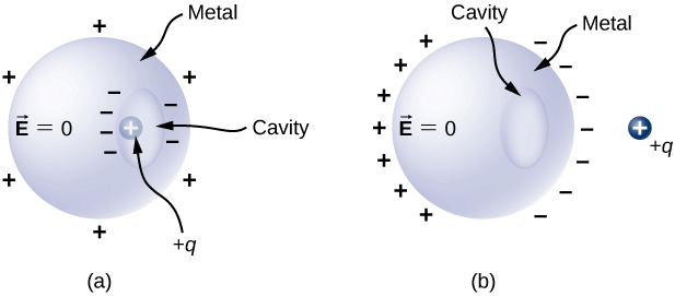
Cavities in Conductors

Suppose we have a conductor with a cavity inside it. If we place the conductor into an external electric field, we know that the conductor will become polarized, as in Fig. \(\PageIndex{2}\). Will the empty cavity become polarized also? The answer is no. Because there is no electric field inside the conductor and no charge in the cavity, there will also be no electric field in the cavity and, therefore, no charge on the surface of the cavity (Fig. \(\PageIndex{8b}\); see Conductors in Electrostatic Equilibrium Via Gauss's Law for additional justification for this claim).

If we put a charge \(+q\) inside the cavity, then the charge separation takes place in the conductor, with \(-q\) amount of charge on the inside surface and a \(+q\) amount of charge at the outside surface (Figure \(\PageIndex{8a}\)). However, the electric field inside the conductor itself will remain zero.

Figure \(\PageIndex{8}\): (a) A charge inside a cavity in a metal. The distribution of charges at the outer surface does not depend on how the charges are distributed at the inner surface, since the \(\vec{E}\)-field inside the body of the metal is zero. That magnitude of the charge on the outer surface does depend on the magnitude of the charge inside, however. (b) A charge outside a conductor containing an inner cavity. The cavity remains free of charge. The polarization of charges on the conductor happens at the surface.