5.2: Consequences and Applications of Induction

Eddy Currents and Magnetic Damping

In our original discussion of motional emf, we pointed out that the bar actually has to be pushed through the magnetic field in order to maintain a constant speed, since the induced current experiences a force that opposes the motion. We noted that this was necessary for energy to be conserved. This same effect can be exploited as a breaking device.

Consider a conducting plate moving through a localized magnetic field (say past the pole of a magnet).

Figure 5.2.1a – A Conductor Swings into a Localized Magnetic Field

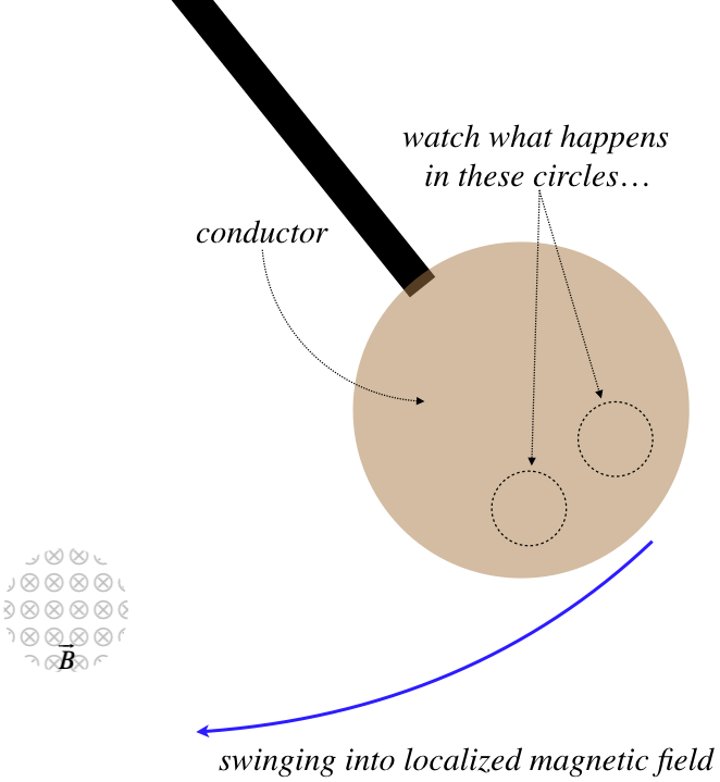
When this conductor reaches the vertical and moving to the left through the magnetic field, the flux through each of these circles is changing in different ways.

Figure 5.2.1b – A Conductor Swings into a Localized Magnetic Field

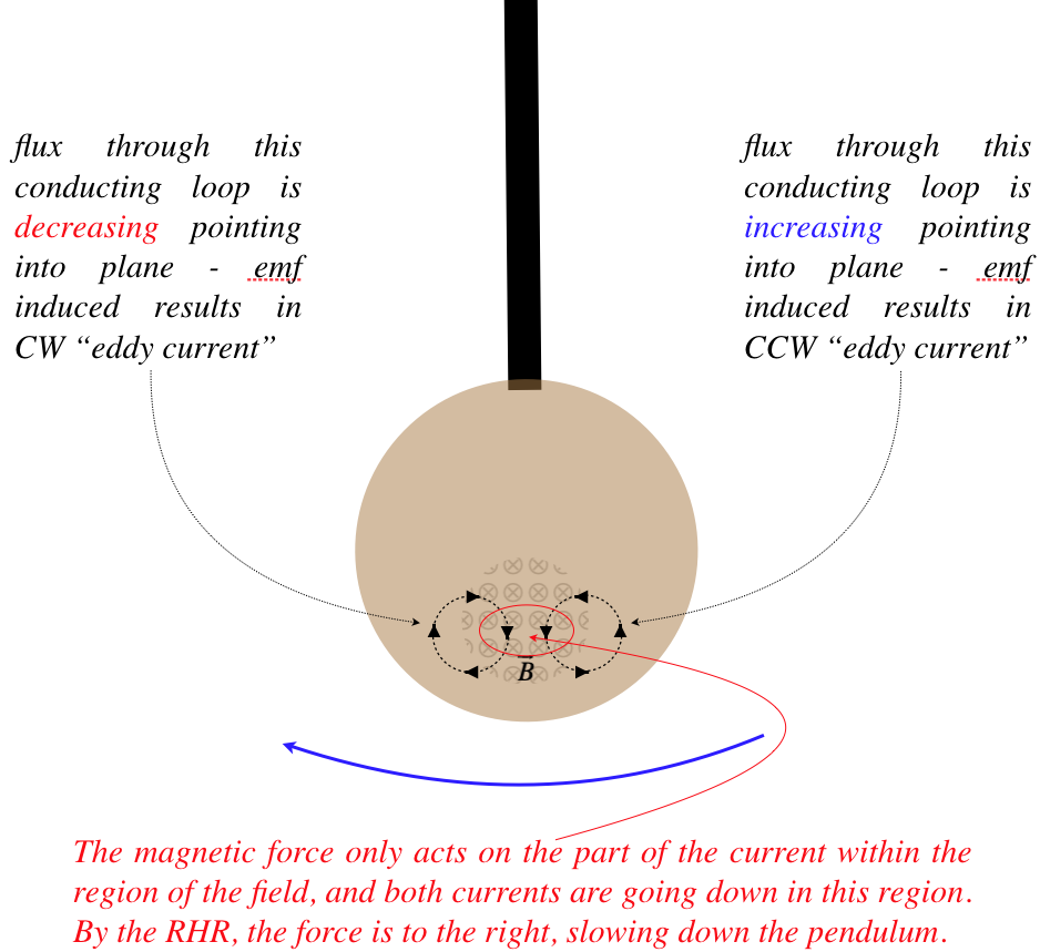
As usual, we find that when currents are induced, the energy they require is removed from the mechanical system inducing that current. These swirly eddy currents that form in the conductor due to magnetic induction (they appear everywhere in the conductor that passes through the field, not just the two spots shown in the figure) also require energy, and as we can see, the magnetic force on these eddy currents acts to damp the motion of the conductor through the field. Ultimately the energy that forms these currents is turned into thermal energy as the current passes through the resistance in the conductor.

Electric Generators

The natural next step to take in magnetic induction is to produce consistent, usable, electrical current. This is done through the use of a device once referred to as a dynamo, and now is generally known as a generator. These come in lots of varieties, but they all ultimately convert mechanical energy (which can come from the potential energy of water falling through a turbine in a dam, the kinetic energy of wind turning a windmill, or a hamster in an exercise wheel) into emf that can drive a current. We will focus here on a couple of designs that result in direct current, though nowadays generators that produce an oscillating alternating current are far more common.

The very first design for such a dynamo was by Faraday himself, and it is essentially a clever way of using the "sliding bar" method of generating motional emf (described in Section 5.1) without the problem of the bar reaching the end of its track. If we fix one end of the bar to a pivot, and spin it in a circle whose plane is perpendicular to a uniform magnetic field, then it can constantly produce a motional emf between its two ends. But Faraday took this one step further: Imagine gluing many thin pie-slice wedges of these bars together so that they form a solid conducting disk, then spin the disk in the field. Then a motional emf will be generated between the center of the disk and its edge. One lead of a circuit can be connected to the center, and the other to a conducting brush that makes contact with the outer edge, and as long as one keeps the disk rotating, current will flow through the circuit.

Figure 5.2.2 – A Faraday Disk Dynamo

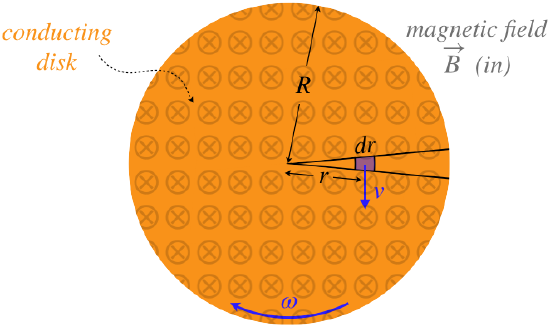
To compute the emf generated between the center and the rim, we consider the small section of conductor (that is the "metal bar" moving through the field). Motional emf is created between the two ends of this segment, with the right-hand-rule telling us that the side farther from the center of the disk will have the higher potential. The length of the bar is \(dr\), so the tiny emf generated is, according to Equation 5.1.1:

\[d\mathcal E = v\;B\;dr\]

The segment is traveling in a circle, so its speed \(v\) is related to its distance from the center and the disk's rotational speed by \(v=r\omega\). The same potential difference exists for every segment of conductor in the pie slice, so these can be added together to get a total potential difference between the center of the disk and its rim. Noting that both \(\omega\) and \(B\) are assumed to be constant, we get:

\[\mathcal E \text{(center to rim)}= \int\limits_{r=0}^{r=R}\left(r\omega\right)B\;dr = \frac{1}{2}R^2\omega B \]

A couple of notes to make here:

• Every pie slice is doing this at the same time, making the entire rim at the same higher potential.
• In the case above, if the dynamo is spun in the opposite direction, or if the field points in the opposite direction, then it would be the center of the disk that would be at the higher potential.
• As always, if a current is flowing thanks to this device, the energy is coming from whatever mechanical energy is keeping the disk turning, which means that there must be a torque opposing the rotation of the disk as the current flows (against which work is being done). If this torque serves to slow the rotation while the current charges a battery, we have all the essential ingredients necessary for regenerative braking currently common in electric and hybrid automobiles.

A nice feature of the disk dynamo is that as long as the rotational speed is held constant, the potential difference is unchanged. The next generator we will look at is a somewhat less cumbersome design than the disk dynamo, but while it does provide a direct current (i.e. a current that doesn't change direction), the emf is not a steady one.

We have seen this other design before – it is identical to that of the DC motor!

Figure 5.2.3 – A Reversed DC Motor is a DC Generator

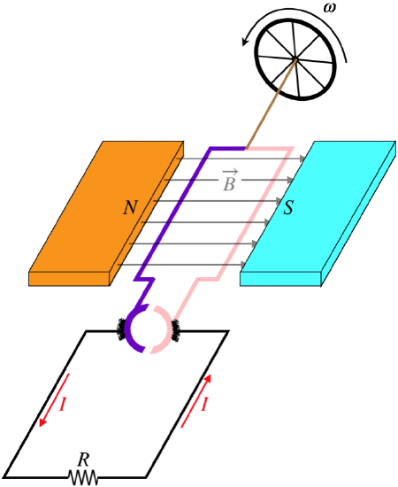
With the wheel being turned at a constant rate, we can use Faraday's law to compute what the induced emf is around the closed circuit as a function of time (we'll compute the absolute value of the emf, and figure out the direction with Lenz's law afterward):

\[\left|\mathcal E\right| = \left|\dfrac{d}{dt}\Phi_B\right| = \left|\dfrac{d}{dt}\left[BA\cos\theta\right]\right|= \left|BA\dfrac{d}{dt}\cos\theta\right| = \left|BA\left[-\sin\theta\dfrac{d\theta}{dt}\right]\right|=\omega B A \left|\sin\theta\right|\]

At the moment depicted in the diagram, the emf is a maximum. We can determine the direction of the induced current by considering what happens to the loop an instant later – the pink side is rising, so the flux is increasing left-to-right through the loop with the pink side above the purple side. The induced current will seek to reduce this increase in flux, which from the right-hand-rule tells us that the emf is induced such that the current will flow up the pink side and down the purple side, giving the direction indicated in the figure.

It is important to note that unlike the disk dynamo, this DC generator does not produce a constant emf (it varies according to \(\sin\theta\)). The presence of the commutator keeps this current always going in the same direction, but it varies from one moment to the next. Many generators like this do not include a commutator, producing alternating current instead. Which generator is used largely depends upon the application. For example, if you want to charge a battery or a capacitor, you don't want the emf constantly changing direction (causing the charge to go into and out of the device you are charging), but if you are turning on a heating element, the resistor will produce thermal energy no matter which way the current is going.

Finally, we will note (as we always do) the fight that goes on between the electrical and mechanical sides of this device. When we are running a motor, the coil is turning in the magnetic field and generating an emf opposite to the direction of the applied emf, reducing the current that goes into driving the motor (this is called back emf). Similarly, when running as a generator, the current generated is in a magnetic field, resulting in a torque that opposes the rotation. This assures that we have to constantly do work to keep the generator running, converting the work added into electrical energy that then accomplishes whatever it is doing.

Diamagnetism

In Section 4.4 we discussed ferromagnetism and paramagnetism, two phenomena that result in materials acting as sources of magnetic fields. The former is responsible for permanent magnets, and the latter for the ability of magnets to stick to otherwise unmagnetized objects like paper clips and refrigerators. These phenomena occurred because dipoles that occur naturally in matter are allowed to align with the external fields.

But another effect also occurs when a magnetic field is introduced to materials. The change of the magnetic flux through the material induces an emf that results in the electrons' average motions opposing the flux according to Lenz’s law. This occurs in everything (even paramagnetic substances), but the effect is much smaller than paramagnetism, so it is much harder to witness, and it doesn’t “undo” para- or ferro- magnetism. Though it is weak, it can be seen in some substances (most notably, water) under the influence of very strong magnetic fields.

There is one way that we can very dramatically witness diamagnetism in action. This involves a substance that allows for a great deal of induced current to be created at the atomic level, due to the very low resistance of the substance. This substance is known as a superconductor, because its resistance is effectively zero. Let’s imagine what would happen if we set a magnet down on a slab of superconductor. The induced current would oppose the new flux, which means that the magnetic field from the superconductor will be in the opposite direction of the applied field, causing a repulsive force, and levitation!

It turns out that this doesn't come close to describing the full story of magnetic effects on superconductors. There is much more that is even stranger (something called the Meissner effect), but a treatment of this topic involves quantum mechanics, and is beyond the scope of this class.

Induced Electric Fields

When we talked about motional emf and moved on to Faraday’s law, we glossed-over the fact that for motional emf we could explain the induced current in terms of forces on particles, but for Faraday’s law we didn’t have a similar explanation. For example, suppose we place a solenoid inside a loop and vary the current. The magnetic field outside the solenoid remains zero, which means it cannot be exerting forces on the charges in the conductor, so how does this induce a current? To answer this, we need to return to where the force on charges in a conductor (causing current) comes from.

If we introduce a battery to a closed circuit, there are really two electric fields involved. One of these is within the battery (produced by the chemical reactions), which acts to separate the free charge inside the battery to the two terminals. The second electric field is the one that is produced by the battery terminals in the conductor through which the electric current flows. If we add up the voltage drops around the full circuit, both of these fields contribute.

Figure 5.2.4 – Voltage Drops Around a Circuit with a Battery

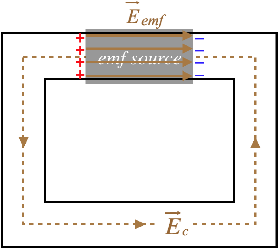
Integrating the electric field around the closed path that is the circuit gives the sum of the voltage drops, and whichever direction we choose for our closed path, one of the electric fields is along the path direction and one is opposite to it. These two contributions cancel to give the usual Kirchhoff loop rule result:

\[\oint \overrightarrow E \cdot \overrightarrow {dl} = \int \limits_{conductor} \overrightarrow E_c\cdot \overrightarrow {dl} + \int \limits_{emf\;source} \overrightarrow E_{emf}\cdot \overrightarrow {dl} = 0\]

But when the source of the current is a changing magnetic flux due to a changing magnetic field strength through a circuit of fixed dimensions, the result is different. There is only one electric field present in this case – the one that drives the current. There is no section of the circuit where an emf source has an opposing field.

Figure 5.2.5 – Voltage Drops Around a Circuit Driven by a Changing Magnetic Field

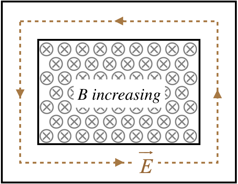
In this case, when we take the same integral around a closed path, we don't have two sections that cancel, and the result is a non-zero integral:

\[\oint \overrightarrow E \cdot \overrightarrow {dl} \ne 0\]

This is agreement with Faraday's "modified Kirchhoff loop rule" explanation, given in Equation 5.1.4. Instead of talking about the changing flux inducing an emf, we can directly relate the magnetic and electric fields in the following way:

A changing magnetic field induces an electric field that circles around it in the direction defined by Lenz's law.

We can now use Equation 5.1.4 to specify this observation mathematically:

\[\text{sum of voltage drops around closed loop} = -\oint \overrightarrow E \cdot \overrightarrow {dl} = \dfrac{d}{dt} \int \overrightarrow B \cdot d\overrightarrow A\]

We can turn this integral equation into a differential equation with the help of Stokes' theorem:

\[\oint \overrightarrow E \cdot \overrightarrow {dl} = \int \left(\overrightarrow \nabla \times \overrightarrow E\right) \cdot d\overrightarrow A \;\;\;\Rightarrow\;\;\; \overrightarrow \nabla \times \overrightarrow E = -\dfrac{d}{dt}\overrightarrow B \]

This is Faraday's law in local (or differential) form.

Back when we studied electrostatics, we noted that the electric field could be written as the negative gradient of the electrostatic potential, and that this meant that the curl of the electric field vanishes (Equation 2.2.13). This is clearly not the case when there is a changing magnetic field nearby, which means that an electric field in this circumstance cannot be written as a negative gradient of a potential field. Indeed, by now we have left electrostatics far behind (we now consider currents flowing all the time), so it isn't surprising that we would lose this special relation.

One last comment here: An electric charge in space (not in a conductor with resistance) that follows a path that traces the electric field that circulates around a changing magnetic field, will be going faster or slower (depending upon the direction relative to the electric field and the sign of the charge) when it gets back to where it started. That is, this is not a conservative force! Not to worry, energy is still conserved overall, because the accelerated charge is not a closed system. Magnetic fields are produced by other moving charges, and for the magnetic field to change, their motions need to change. Together this interplay forms a very complex dance, and careful accounting of all the energy shows that it does remain constant for the whole system.