3.4: Energy Accounting with Conservative Forces: Potential Energy

Internal Forces

We have discussed how work done on a object (a collection of particles) can contribute to both the overall kinetic energy of that object (measured using its total mass and the speed of its center of mass) and the internal energy of the object. But our definition of internal energy as the sum of the kinetic energies of the particles in the center of mass frame is not very robust. For example, suppose that the particles within an object exert forces on each other, as they do in pretty much every object except for a container of ideal gas.  This will change the kinetic energies of the particles, and according to our current definition of internal energy, it will change. Implicit in the name "internal energy" is the idea that it is a fixed quantity unless some outside influence changes it.  It would be nice, therefore, to somehow account for the effects of the internal forces so that we have an intuitively-defined internal energy.

Conservative Forces Provide a Shortcut

One thing that the internal forces between individual particles have going for them is that they are conservative. We have learned that when forces with this property do work on a particle as it moves from point \(A\) to point \(B\), it doesn't matter what path the particle takes in that journey. This actually allows us to introduce a significant shortcut when dealing with conservative forces. Consider the following situation...

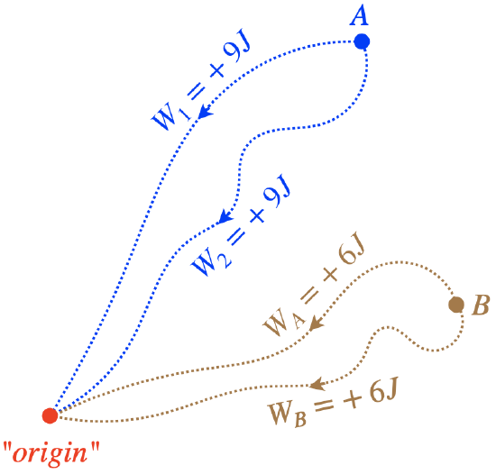
Suppose we have a conservative force that is well-defined by the location of the particle on which it acts. That is, at every point in space, there is a well-defined force vector \(\vec F\left(x,y,z\right)\). Let's start by choosing, completely arbitrarily, a point in space that we call the "origin." Next, we will place a particle at some other position in space (position "\(A\)", and move it from that position to the origin through some arbitrary path, adding up the work done on the particle as we do (i.e. performing the line integral for the force from \(A\) to the origin). We know that since the force is conservative, if we had chosen a different path between these two points, we would have computed the same work done by the force. Let's repeat this for a new starting point (position "\(B\)"). Once again we find that we can follow any path from \(B\) to the origin and the work done would be the same.

Figure 3.4.1 – Work Done Coming to the Origin

Given that it doesn't matter what path is taken from any given point in space, we can save ourselves a lot of trouble by just labeling every point in space with the energy value that equals the work the force would do in moving the particle from that point to the origin. Then whenever a particle is moved from a point in space to the origin, we would immediately know how much its kinetic energy changed, without having to even think about doing a line integral. Note that the origin would automatically be labeled with a zero energy value.

Figure 3.4.2 – Labeled Points in Space

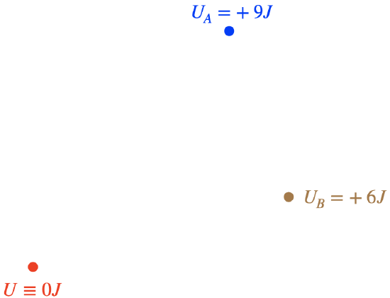
Now whenever a particle is at one of these points in space, one might say that the force "provides the potential to change the particle's kinetic energy by an amount equal to the value at that point, if it is moved to the origin." Not coincidentally, these values are known as potential energies. As we have seen here, the value of a potential energy at a point in space depends upon two things: The conservative force that is involved, and the position chosen to be the origin (which we will hereafter refer to instead as the "position of zero potential energy", as the word "origin" has coordinate system implications).

This would seem to have limited use, as it only applies to a very specific ending point of the journey of the particle. But actually this trick is more robust than this. Consider the case of a particle again moved from \(A\) to the origin above, but this time let's chose a path that passes through \(B\).

Figure 3.4.3 – Path from A to Origin Through B

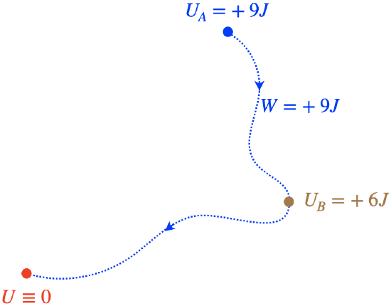
Like any other path to the origin, this one comes with a work done on the particle equal to the potential energy at point \(A\). But the work done by the force during the part of the trip from \(B\) to the origin contributes an amount of work equal to the potential energy at point \(B\), and this tells us something about the work done in going from point \(A\) to point \(B\), neither of which is the origin.

Figure 3.4.4 – Work Done from A to B

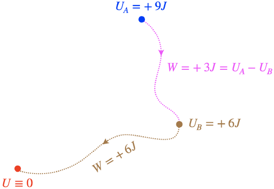
It's also to important to note that the work done from point \(A\) to point \(B\) doesn't depend at all upon where we placed the origin.  The second leg of the trip shown above from point \(B\) to the origin could have gone to any origin whatsoever, and the work done from \(A\) to \(B\) would still come out the same. We therefore claim, more generally, the following:

The work done by a conservative force acting on a particle that moves from point A to point B equals the amount that the potential at those points drops as a result of the trip.

\[W\left(A\rightarrow B\right) = U_A - U_B = -\left(U_B - U_A\right) = -\Delta U\]

Here we have adopted the usual meaning of "\(\Delta\)" meaning "after minus before". There are a few important things to emphasize here:

• If the particle returns to where it started, then the difference is between the same two numbers, giving zero. As we have already seen, for a conservative force, the work done over a path that returns to its starting point is indeed zero.
• Once we have arbitrarily chosen an origin (zero potential energy) to be a given point in space, then the potential energy values of all the other points in space are well-defined. Actually, we do not need to even have zero potential be our starting point – fixing any value for potential energy at a specific point in space will define all of the potential energies just as well. When we introduced kinetic energy, we pointed out that we can't say that a particle or collection of particles "has" a specific kinetic energy, without first defining the reference frame of the observer of that kinetic energy. Potential energy has a similar ambiguity: We can't say that a particle "has" a specific potential energy without first clarifying what we have chosen as our arbitrary reference position & value for the potential energy.
• The potential energy values defined in space are only for the specific conservative force in question. The particle may have several forces on it, and some may not be conservative. This shortcut can still be used for the individual conservative force's work contribution, but not for all the forces combined (unless the combination of all the forces happens to make a conservative composite force). Non-conservative forces do not provide us this opportunity – there is simply no way to define a potential energy for forces like kinetic friction.

Digression: Fields

The idea of associating a value with every point in space is one that comes up frequently in physics. These values and the positions to which they are assigned are collectively referred to as a field. If the values associated with each point in space are simply numbers, as they are for potential energy, then it is called a scalar field. It's also possible to assign a vector at each point in space (say, for example, the velocity of the particle at every point in space filled by a gas), and this is called a vector field. We will deal much more with fields in future physics classes, especially Physics 9C.

When the particle moves from a higher potential energy to a lower one, positive work is done, which means the kinetic energy rises. Potential energy can be thought of as a bank balance - work has the effect of either "spending" the balance, moving that potential energy into the kinetic energy of the particle), or "storing" the balance, taking kinetic energy away and adding it to the potential energy balance. If we are talking about particles or objects on which there are only conservative forces acting, then every change in its total potential energy is balanced by an opposite change in its kinetic energy – the sum of these two numbers remains constant. Whenever we run across a quantity that remains fixed despite a change in circumstances, we can that this quantity is conserved. If only conservative forces are present, then:

\[0 = \Delta U + \Delta KE = \Delta\left(U + KE\right)\]

The quantity \(U+KE\) is conserved (unchanging) provided that there are only conservative forces present, and that these forces are represented by potential energy functions. This quantity is commonly known as mechanical energy.

Potential Energy for Collections of Particles

It might seem like the use of potential energy would be very limited, given that it is only defined for conservative forces, and as we have seen, when many particles are involved, the force on a single particle can easily be non-conservative.  In the previous section, we mentioned the example of a three "particle" collection of the Sun, Jupiter, and the Voyager probe where the latter "particle" experienced a combined force from the other two that was not conservative. The reason that the force on the voyager probe is non-conservative is that when the gravitational forces from the Sun and Jupiter do work on Voyager, those same forces also do work on the Sun and Jupiter! So the kinetic energy gained by the probe from the other two bodies is energy lost by those other bodies.  Put another way, the Sun + Jupiter combination loses exactly the same amount that the kinetic energy that Voyager gains.

It turns out that if we consider all of the particles in the collection together, and we add up the kinetic and potential energies of all the particles combined, then this number for the grouping (assuming no external work comes in) remains fixed (conserved).  The way we compute the potential energies is pairwise – every possible combination of two particles has a fundamental force between them, and therefore a well-defined potential energy.  So the total potential energy of the Sun+Jupiter+Voyager combination is the sum of the gravitational potential energies of Sun+Voyager, Jupiter+Voyager, and Sun+Jupiter.  When you also add in their kinetic energies, you get a total energy for the collection that remains conserved. The apparent weirdness comes from the fact that these three bodies can re-partition the energy in unexpected ways (so that Voyager gains a lot of KE, for example).

Because this scheme for adding potential energies pairwise between particles in a collection assures that the total energy of the grouping remains unchanged, we are able to make the following powerful claim:

The total energy of any isolated collection of particles remains conserved.

\[\Delta E_{tot}=\Delta\left(\sum KE_i+\sum U_i\right)=0\]

Naturally if the collection is not "isolated," external bodies can exert forces that do work on the particles, thereby adding energy to, or taking energy away from the collection.  But the internal forces within the group of particles that do work only serve to exchange kinetic and potential energy between the particles within the group, thereby leaving the total energy unchanged.

There is one bit of clarification needed for the equation above.  The index \(i\) is obviously intended to run over all of the particles in the collection. The quantity \(U_i\), or "potential energy of the \(i\)th particle" really involves all of the particles, because the potential energy values are determined from pairwise forces between particles. So the value of \(U_i\) is really a sum of potential energies between particle \(i\) and particle 1, particle \(i\) and particle 2, and so on.

Energy Accounting For Conservative Forces

We now know two alternative ways to account for what changes the kinetic energy of a particle or collection of particles (macroscopic object). What differs between these choices is the definition of something we will call a system. A system is simply a well-defined collection of objects (in most cases we will be discussing from now on, these will not be single particles). Energy is transferred into or out of a system through work done by forces exerted by objects outside the system. Objects within the system that exert forces on each other keep the energy in the system, though it can change forms.

Figure 3.4.5 – Changing Energy Accounting for Conservative Forces

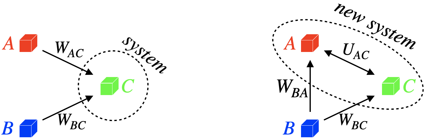
The figure above shows a physical situation where three objects are interacting with each other through conservative forces. On the left, we have chosen just object \(C\) as our system and the forces from the other two objects do work on this object, exchanging energy with the system. The left diagram employs exclusively the work-energy theorem – the work from the external forces changes the kinetic energy of object in the system.

One the right is the same physical situation, but we have changed our accounting method. We have extended what we have defined as a system to include one of the other two objects. As the forces involved were conservative, we can account for the interaction between objects \(A\) and \(C\) using potential energy. This energy is entirely contained within the system, where it can be exchanged freely with the kinetic energies of objects \(A\) and \(C\). Object \(B\) has been left outside the system, so accounting for its contribution to the system's energy still relies upon computing work.

Notice that in our definition of system as only object \(C\), we didn't care at all about the interaction between particles \(A\) and \(B\) in our accounting, but once object \(A\) was brought into the system, this interaction became relevant, because the energy exchange is now across the system border.

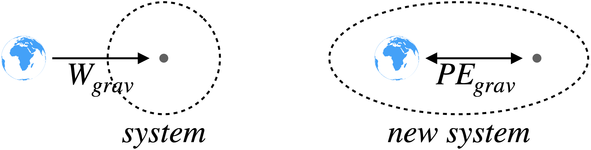
Given the difficulty of computing line integrals, we will generally pull all of the objects into the system that are exerting conservative forces, so that we can use the potential energy "shortcut." Let's look at a concrete example – gravity.

Potential Energy Function for Gravity

Even though it is not a force between two individual particles, the force of gravity by the Earth on an object like a stone is (to an extremely good approximation) conservative. As discussed above, we can choose to do the energy accounting for a falling stone by putting making the stone the system and computing the work done on the stone by the Earth, or we can include the Earth in the system and compute the potential energy change of the Earth/stone system as the stone falls.

Figure 3.4.6 – Energy Accounting for Gravity

In Equation 3.3.11, we computed the work done by the gravity force on a projectile, and found:

\[ W_{grav} \left( A \rightarrow B \right) = - mg \left(y_B-y_A\right)=mgy_A-mgy_B \]

Above we said that the work done from point \(A\) to point \(B\) is the potential energy at point \(A\) minus the potential energy at point \(B\), so it seems clear that we can define the potential energy function for gravity (near the Earth's surface) as:

\[ U_{grav}\left(y\right) = mgy \]

But this definition implies that we have already determined a position where we have defined \(y=0\). We can of course choose our arbitrary reference point to be whatever we like, so it can be useful to express this in the equation. We therefore have:

\[ U_{grav} \left( y \right) = mgy + U_o, \]

where \(U_o\) is an arbitrary constant. Notice that if we take a difference of potential energies at two different altitudes, the constant drops out, showing that its actual value doesn't change the physics:

\[ \Delta U_{grav} = U \left( y_B \right) - U \left( y_A \right) = \left( mgy_B + U_o \right) - \left( mgy_A + U_o \right) = mg \left(y_B - y_A \right) = mg \Delta y \]

Analyze This

There are few things as fun as swinging into a river from a rope swing tied to the limb of a tree on its banks. The person at the end of this rope starts at the top of a hill at one angle, then swings to another angle when they let go and fly into the water.

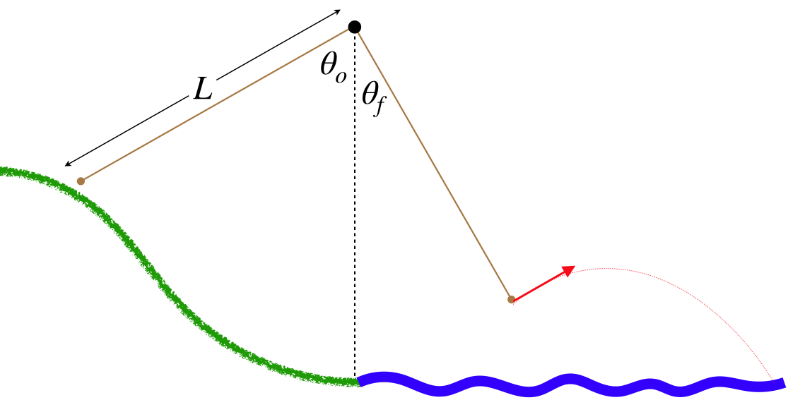
Analysis

The tension of the rope does no work here, as it acts perpendicular to your motion throughout. Ignoring air resistance, we therefore can use the total energy conservation of the swinger to determine the change in the swinger's speed from the point where they leave the ground to the point where they release the rope (the swinger is an object that is collection of many particles, but we assume that none of the total energy referred to here is going into the swinger's internal energy):

\[0 = \Delta U_{grav} + \Delta KE\nonumber\]

The potential energy here is due to gravity, so we need to know the change in height from the start to the end. This requires some geometry to figure out. The simplest approach is to use the right triangles the rope makes with the vertical and horizontal directions, and measure the distances below the tree limb. Calling the height of the tree limb zero, we have:

\[ \left. \begin{array}{l} \text{start:} && y_o = -L \cos \theta_o  \\ \text{end:} && y_f = -L \cos\theta_f \end{array} \right\} \;\;\; \Rightarrow \;\;\; \Delta U_{grav} = mg \left(y_f - y_o \right) = mgL \left( \cos \theta_o-\cos \theta_f \right) \nonumber \]

Putting this into total energy conservation gives:

\[ 0 = \Delta U_{grav} + \Delta KE = mgL \left( \cos \theta_o-\cos \theta_f \right) +\left(\frac{1}{2} mv_f^2 - \frac{1}{2} mv_o^2 \right) \;\;\; \Rightarrow \;\;\; v_f = \sqrt{v_o^2 - 2gL \left( \cos \theta_o-\cos \theta_f \right)}\nonumber \]

Potential Energy Function for Elastic Force

For the case of an object pushed or pulled by a spring, we can again choose only the object as a system and compute the work done by the spring force, or include the spring in the system and use the change in its potential energy. For the a stretched or compressed spring with the \(x\) variable defined to be zero when the spring is at its equilibrium length, we obtained Equation 3.3.14:

\[ W_{spring} \left( A \rightarrow B \right) = - \frac{1}{2} k \Delta \left( x^2 \right) = \frac{1}{2} kx_A^2-\frac{1}{2} kx_B^2\]

As with the case of gravity, this immediately implies a function for elastic potential energy:

\[ U_{elastic}\left(x\right) = \frac{1}{2}kx^2 +U_o \]

If we return to the more general case of the position of the spring at equilibrium being \(x_o\), then to get the proper potential energy function, we only need to make the substitution \(x \rightarrow x-x_o \), giving:\[U_{elastic} \left( x \right) = \frac{1}{2}k \left(x-x_o \right)^2 + U_o \]

The Formal Relationship Between Potential Energy and Force

Given the close ties between work done by a conservative force and the potential energy function for that force, we must be able to link force to potential energy more formally. If we take Equation 3.4.1 and rewrite it using the definition of work, we get:

\[ U_B - U_A = -\int \limits_A^B \overrightarrow F \cdot \overrightarrow {dl} \]

The whole idea of using potential energy is to be able to express it as a function of position, so the question that arises is, "Is there some way to 'reverse' this equation, so that if we are given the potential energy function, we can determine the force function?" Well, we already know the answer to this: The 'reverse' of an integral is a derivative! This is the Fundamental Theorem of Calculus. Reversing a line integral is a little bit trickier than doing it for the simple single-variable integrals we are used to from our basic calculus classes, but it can nevertheless be done. To see how this works, let's consider only a very tiny change in potential energy due to a very small displacement. This changes the left hand side of our equation to an infinitesimal, and the right hand side is no longer a sum of many pieces, but is instead only a single piece:

\[ dU = -\overrightarrow F \cdot \overrightarrow {dl} \]

In three dimensions, the tiny displacement can be written as:

\[ \overrightarrow {dl} = dx \; \widehat i + dy \; \widehat j + dz \; \widehat k \]

This means that the dot product with the force vector is:

\[ \overrightarrow F \cdot \overrightarrow {dl} = F_x dx + F_y dy + F_z dz \]

Suppose we make our tiny displacement only along the \(x\)-axis, so that \(dy\) and \(dz\) are zero. Then clearly all the work done by the force is given by the first term above, and we get that the small change in potential energy that occurs when the position changes a small amount in the \(x\)-direction is:

\[ dU \left(x \rightarrow x+dx \right) = -F_xdx \;\;\;\Rightarrow\;\;\; F_x=-\dfrac{dU}{dx} \]

This is fine for a potential that changes only in the \(x\)-direction, but what happens if the potential energy is also a function of \(y\) and \(z\)? The answer is that we treat \(y\) and \(z\) as though they are constants, which means that \(dy = dz = 0\), and our result above works. When we treat \(y\) and \(z\) as constants, we have to return to the partial derivatives we discussed in Section 3.3. We therefore have the following relationship between the potential energy function and the force components:

\[ F_x = -\frac{\partial}{\partial x} U, \;\;\; F_y = -\frac{\partial}{\partial y} U, \;\;\; F_z = -\frac{\partial}{\partial z} U \]

Digression: Gradient

As was the case with the curl digression in Section 3.3, a reader that is further along in math than most will recognize this relationship between the scalar function \(U\left(x,y,z\right)\) and the vector function\(\overrightarrow F\left(x,y,z\right)\) as that of a (negative) "gradient":

\[\overrightarrow F =-\frac{\partial U}{\partial x}\;\hat i-\frac{\partial U}{\partial y}\;\hat j-\frac{\partial U}{\partial z}\;\hat k \equiv -\overrightarrow\nabla U= \text{negative gradient of }U\left(x,y,z\right)\nonumber\]

Exercise

We know that a potential energy function can only exist for a force that is conservative. It is a mathematical fact that multiple partial derivatives of a single function can be performed in any order.  That is, if the partial derivative of the function \(f\left(x,y\right)\) with respect to \(x\) is taken, followed by a partial derivative of the result with respect to \(y\), then the same result is obtained if the partial derivatives are performed in the opposite order. Use this mathematical property to show that Equation 3.4.17 produces a conservative force from the potential energy function.

Solution

We already have a check for a conservative force – Equation 3.3.8. If we apply this to the \(x\) and \(y\)-components of the force given by Equation 3.4.15, we get:

\[\dfrac{\partial}{\partial x}F_y-\dfrac{\partial}{\partial y}F_x=\dfrac{\partial}{\partial x}\left(-\frac{\partial U}{\partial y}\right)-\dfrac{\partial}{\partial y}\left(-\frac{\partial U}{\partial x}\right)=0\nonumber\]

The mathematical property of the reversibility of partial derivatives was used in the final equality.

Exercise

Show that the partial derivative link between the potential energy function works for the two macroscopic conservative forces we have discussed:

1. gravity:    \(U_{grav}\left(x,y,z\right)=mgy + U_o\)
2. elastic:    \(U_{elastic}\left(x,y,z\right)=\frac{1}{2}kx^2 + U_o\)

Solution

Just plug-in and turn the crank in each case:

a. gravity:

\[\left.\begin{array}{l} F_x=-\frac{\partial}{\partial x}\left(mgy + U_o\right)=0 \nonumber \\ F_y=-\frac{\partial}{\partial y}\left(mgy + U_o\right)=-mg \nonumber \\ F_z=-\frac{\partial}{\partial z}\left(mgy + U_o\right)=0\nonumber\end{array}\right\}\;\;\;\overrightarrow F = -mg\;\hat j\nonumber\]

a. elastic:

\[\left.\begin{array}{l} F_x=-\frac{\partial}{\partial x}\left(\frac{1}{2}kx^2 + U_o\right)=-kx \nonumber\\ F_y=-\frac{\partial}{\partial y}\left(\frac{1}{2}kx^2 + U_o\right)=0 \nonumber\\ F_z=-\frac{\partial}{\partial z}\left(\frac{1}{2}kx^2 + U_o\right)=0\nonumber\end{array}\right\}\;\;\;\overrightarrow F = -kx\;\hat i\nonumber\]

Analyze This

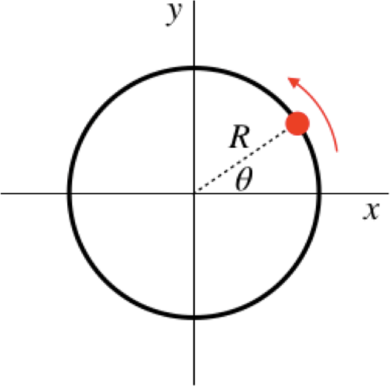
A bead is threaded onto a frictionless circular loop that lies in the horizontal \(x\)-\(y\) plane, as shown in the diagram below. This bead is subjected to a conservative force that is characterized by the potential energy function:

\[U\left(x,y\right)=-\alpha\left(Rx+y^2\right)\;\;\;\;\;\alpha > 0\nonumber\]

Analysis

The loop of wire is frictionless, so it can only produce a force that lies perpendicular to the circle (i.e. radially inward or outward). With the bead only allowed to move along the circle, this means that the loop can do no work on the bead. Also, with the loop being in a horizontal plane, the bead never changes elevation, so gravity will not do any work either.  This means that the only force acting on the bead is the one that comes from the potential energy function given. The obvious next step is to determine this force, which we do with the partial derivatives:

\[F_x=-\frac{\partial U}{\partial x} = \alpha R \;\;\;\;\; F_y=-\frac{\partial U}{\partial y} = 2\alpha y \nonumber\]

So the component of the force along the \(x\)-direction remains constant, while the component along the \(y\) direction grows stronger as the magnitude of the \(y\) value gets larger.  We can therefore immediately determine the positions on the loop where this potential field exerts the strongest force. It does this when the bead crosses the \(y\)-axis, and at these points, the magnitude of the force from the potential field is:

\[F_{max}=\sqrt{\left(\alpha R\right)^2+\left(2\alpha R\right)^2}=\sqrt{5}\;\alpha R\nonumber\]

We know that since the applied force is conservative, when the bead does a complete circle around the loop, it must return to the same kinetic energy at which it started. This means that it can't continually speed up in the same direction, though the direction of the tangential acceleration can flip from clockwise to counterclockwise, or vice-versa. It must make such a flip in a smooth, continuous way, so there must be at least two positions on the loop where the (tangential) acceleration is zero (one where it changes from clockwise acceleration to counterclockwise, and one where it changes back). At such positions, the entire acceleration vector must point radially (no component tangential). The loop already supplies a radial force, so we are looking for the positions where the potential field's force is also purely radial. So let's look for the positions (\(\theta\) values) at which angles result in zero tangential force.

The force from this potential field will point radially when the tangent of the angle it makes equals plus-or-minus the tangent of the angle the position vector makes.  These tangents are simply the ratios of the \(y\) and \(x\) components, so we have:

\[\frac{F_y}{F_x} = \tan\theta\;\;\;\Rightarrow\;\;\; \tan\theta=\frac{2\alpha y}{\alpha R} = 2\frac{y}{R}\nonumber\]

The \(y\)-position divided by the radius of the circle equals \(\sin\theta\), so:

\[\frac{\sin\theta}{\cos\theta}= 2 \sin\theta\;\;\;\Rightarrow\;\;\; \sin\theta = 0\;or\;\cos\theta=\frac{1}{2}\nonumber\]

There are many angles for which one of these conditions exists. Solving these shows that it is true at \(\theta=0^o,\;\pm 60^o,\;and\;180^o\).

It should also be noted that wherever the force changes direction, the bead goes from a state of either speeding-up to slowing-down, or vice-versa, which means that the speed of the bead either hits a local maximum or minimum at these positions. Given that the total energy of the bead remains conserved, low points of potential energies must correspond to high point of kinetic energies (and therefore speeds), and vice-versa.  So looking at each of these critical points we find:

\[U\left(\theta=0^o\right)=U\left(R,0\right)=-\alpha R^2\nonumber\]

\[U\left(\theta=180^o\right)=U\left(-R,0\right)=+\alpha R^2\nonumber\]

\[U\left(\theta=\pm 60^o\right)=U\left(\frac{1}{2}R,\pm\frac{\sqrt{3}}{2}R\right)=-\alpha R^2\left(\frac{1}{2}+\frac{3}{4}\right)=-\frac{5}{4}\alpha R^2\nonumber\]

So it appears that the bead reaches its maximum speed at \(\theta=\pm 60^o\), and its minimum speed at \(\theta=180^o\).

Equipotential Surfaces

Suppose a particle is under the influence of a single conservative force. At a given point in space, the force exerted on the particle has a specific direction. If the particle is displaced slightly in a direction perpendicular to this force vector, then this force will do no work. If no work is done by the force, then the potential energy due to that conservative force could not have changed.  Suppose now we keep displacing the particle from place-to-place, always moving in a direction perpendicular to the force. The region mapped out by all of this moving of the particle will be a surface throughout that region of space, and the force vector at every point on this surface will be perpendicular to it. The potential energy at every point on this surface is the same, and for this reason such a surface is called an equipotential surface. Here's an example:

\[ U\left(x,y,z \right) = -\alpha \left(x^2+y^2+z^2\right) \]

The sum of the squares of the \(x\), \(y\), and \(z\) coordinates is just the square of the distance from the origin. So any sphere that we choose that is centered at the origin will have the same potential at every point on it – these spheres are equipotentials.

We claimed that the force vectors at every point on an equipotential surface is perpendicular to that surface, and we can check that for this example:

\[ \overrightarrow F = \widehat i \; \left(-\dfrac{\partial U}{\partial x}\right) + \widehat j \; \left(-\dfrac{\partial U}{\partial y}\right) + \widehat k \; \left(-\dfrac{\partial U}{\partial z}\right) = 2 \alpha \left( x \widehat i + y \widehat j + z \widehat k \right) \]

Hopefully you recognize the part of this vector in parentheses. It is the position vector relative to the origin, Equation 1.6.1. This vector points directly to the point \(\left(x,y,z\right)\) from the origin, which means that it is perpendicular to the sphere centered at the origin that contains that point, confirming the general property that the force vectors in space associated with a potential are perpendicular to the equipotential surfaces everywhere.

Notice that for the function \(U \left( x,y,z \right)\) above, if \(\alpha>0\), the potential energy gets smaller as one gets farther from the origin, and the force vector from this potential points away from the origin. This is also a general feature – the force associated with a potential points in the direction from greater potential to lower potential. It should be clear on many fronts why this must be the case. If an object moves from a region of higher potential to one of lower potential, this decrease in potential energy must be balanced by an increase in kinetic energy, which means the object speeds up. Objects speed up when the net force on them points in the same direction that they are moving, so the force must point from where the potential energy is higher to where it is lower.