
3.5: Energy Accounting with Non-Conservative Forces: Thermal Energy


- Last updated
- Apr 18, 2023
- Save as PDF

( \newcommand{\kernel}{\mathrm{null}\,}\)
Energy Accounting for Non-Conservative Forces
Okay, so we have seen how we can pull conservative forces due to macroscopic objects into a system and change the accounting to using the simpler potential energies, but what about the case of work done by an external macroscopic object in the case where the force is not conservative? As we have seen already in such cases, we can still account for the total energy if the internal energies are included in the tally. The schematic diagram is only a bit different from the case of the conservative force.
Figure 3.5.1 – Changing Energy Accounting for Non-Conservative Forces
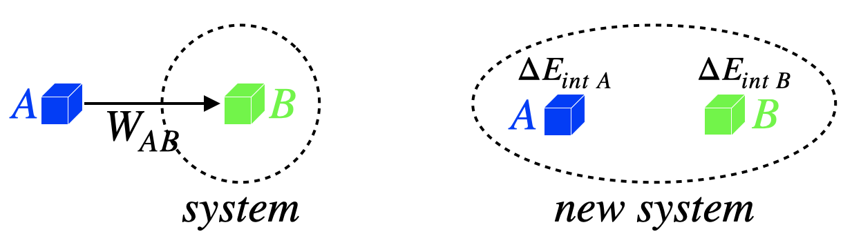
In this case, the external non-conservative force does not allow for redefining the system with a potential energy. Instead, the transfer of energy can only be accounted-for in terms of the internal energies of the objects involved. The change of accounting from the work-energy theorem to the new system therefore looks like:
WAB=ΔKEB⇒ΔKEA+ΔKEB+ΔEintA+ΔEintB=0
This rather abstract description is difficult to wrap one's mind around without a clear example, as gravity was for the conservative force case. So we'll demonstrate how this accounting works with the most common example of a non-conservative force – kinetic friction. We want to keep this as simple as possible, so we will consider the following scenario...
The system in this example consists of two books. They are sliding across a horizontal tabletop, but the tabletop is frictionless, so it exerts no horizontal force on the books. The tabletop does exert a vertical force (the normal force) upward on the books, but as the books do not displace vertically, this force does no work. The Earth also exerts a force (gravity) on the books, but again, as they do not displace vertically, this force does no work either. So despite the presence of the tabletop and the Earth's gravity, the two books really are an isolated system, with no external work done on them (we also assume no air resistance during their motion). Below is a diagram of what occurs between the two books: At first they are separate, and then book A slides on top of stationary book B, the kinetic friction force between them causing book B to speed up and book A to slow down, until they eventually stop rubbing across each other and slide away together at the same speed.
Figure 3.5.2 – Energy Accounting for Kinetic Friction
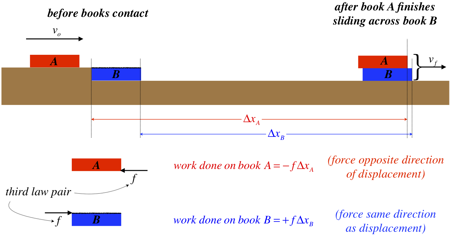
If we treat book B as a system, then the (non-conservative) friction force exerted on it by book A does external work, leading to a change in the kinetic energy of the system:
WAB=+fΔxB=ΔKEB=KEBf−KEBo=12mBv2f−0
If we instead treat both books as a system, then we need to include both of their kinetic energies and their internal energies, and we get the same result as is expressed in Equation 3.5.1. The changes in the kinetic energies of the two books are equal to the works done on each, expressed in the diagram. There are two important things to note here. First, the change in the kinetic energy of book A is negative (it slows down), and this is evident from the work done on it by book B, since the kinetic friction force is in the opposite direction of book A's displacement. Second, the positive work done on book B (and therefore its kinetic energy change) is a smaller magnitude than the negative work done on book A (equal to its kinetic energy change), since they experience forces of equal magnitude (Newton's 3rd Law), and book A displaces farther than book B during the time that they are rubbing against each other. The upshot of these facts is that the quantity ΔKEB+ΔKEA is a negative number. This in turn requires that the changes of internal energy of the two books is positive – they collectively gain internal energy. This is manifested microscopically as an increase in the kinetic and potential energies of the particles in the books, a phenomenon we will address shortly.
We can't compute the change in internal energy of an individual book, but the combined increase in their internal energies can be expressed in terms of what is given in the diagram:
ΔEintB+ΔEintA=−(ΔKEB+ΔKEA)=−fΔxB+fΔxA=f(ΔxA−ΔxB)
The quantity ΔxA−ΔxB is the distance that book A slides across book B, and it is a positive number, which means that there is an increase in the internal energies of the two books. This makes sense, as it means that the amount of energy that goes into the internal energies of the books is a measure of the number of interactions between molecules at the surfaces of the books, and the distance that they slide across each other is directly related to the number of molecular interactions.
There is still much more we can do with this simple two-book model, and we will return to it in a future chapter.
Thermal Energy
There is one subset of the internal energy category that deserves special mention. In most macroscopic model calculations, the internal energy change that occurs in the system comes in the form of random motions of molecules in the participating objects. When two surfaces slide across each other with kinetic friction, the surface molecules push and pull against each other, and as they are bound to their respective objects, they react by vibrating. These vibrations are not in-sync – they are quite random, and the vibrations spread to their neighbor molecules as well. Such vibrating particles possess energy, both kinetic and potential (the latter due to the potential energy from the restoring Van der Waals forces), and this energy is within the objects themselves, so it is internal. This microscopic, random internal energy is so important that it is given its own name – thermal energy.
As is implied by the name, thermal energy is measured most easily through temperature – the two sliding books above become warmer. We will wait until Physics 9B to see how thermal energy and temperature are mathematically related to each other. For the purposes of this class, knowing that a change in temperature is an indication of a change in internal energy will be sufficient. One other important feature of thermal energy that we will not explain until Physics 9B is that with models like the sliding books, the conversion of some of a book's kinetic energy into thermal energy is a one-way trip. We would have a wait a long time if we ever wanted to see the two books cool off and spontaneously slide off each other. This comes from the fact that all (or a very large majority) of the randomly-moving momlecules would have to synchronize and move in the same direction at the same time, and this is improbable in the extreme.
Alert
While it will be some time before you encounter the idea of "heat" in Physics 9B, it is important to understand as early as possible that thermal energy is not the same as heat. Heat is not a form of internal energy.
To get some sense of how important thermal energy is to this discussion, it should be noted that it requires quite a contrived situation to produce an example in the mechanics of macroscopic objects where internal energy is not thermal energy. Indeed, for this reason, most textbooks don't even make the distinction, and instead go straight to the total energy conservation equation:
0=ΔKE+ΔU+ΔEthermal
Thermal energy can have different intrinsic properties for different physical systems. For example, for a system that is a gas, the particles don't interact very much, which means there is very little potential energy included in such a system's internal/thermal energy. For a solid, on the other hand, the molecules are bound to each other, so the energy is divided pretty equally between the potential energies of the particle interactions and the kinetic energies of their motions.
Summary of Energy Accounting
In the last two sections, we have talked about a dizzying number of ways that we can keep track of the energy accounting for a physical system, so let's get away from all the conceptual discussion and summarize what is most useful for solving problems. As a general rule, we will be dealing with systems involving macroscopic objects whose internal energies are all thermal. Aside from these thermal energies, all of the remaining energy will be mechanical. This means that what we will mainly need for any problem are two things: The equation for total energy conservation, and the ability to compute a change in thermal energy by performing the work integral for the non-conservative (usually kinetic friction) force:
0=ΔKE+ΔU+ΔEthermal,ΔEthermal=−Wf=−B∫Af⋅dl
Some important/useful notes:
- There could be more than one type of potential energy present at the same time (such as a spring and gravity), so keep in mind that the "ΔU" in the formula above is a placeholder for all of them summed together.
- We are assuming here that the objects in the system are rigid and are not rotating, so that the kinetic energy for each object is simply 12mv2. This allows us to not be concerned about the specifics of each object's center of mass motion, as every part of it is moving at the same speed. We will see how to deal with the kinetic energy associated with rotational motion in a future chapter.
- It is often helpful to break down the Δ's into "before" and "after", rewriting the energy conservation equation this way:
KEbefore+Ubefore=KEafter+Uafter+ΔEthermal
The interpretation of this equation is a simple one: The system begins with some total energy that is in the form of mechanical energy. Later, the distribution of this total energy has changed. The amount of kinetic and potential has changed, and assuming there was also a non-conservative force present, some of that starting energy has become thermal energy, internal to the objects. Naturally the system started with some thermal energy, and we could similarly divide that between the two sides of the equation, but this equation is used for specific calculations, and while it is possible to compute the thermal energy change using a work integral, it is not possible (in Physics 9A) to compute the thermal energy of an object directly.
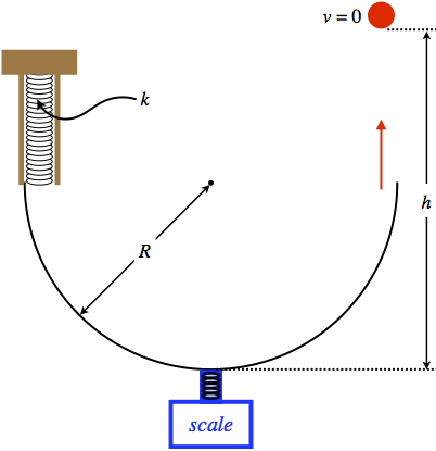
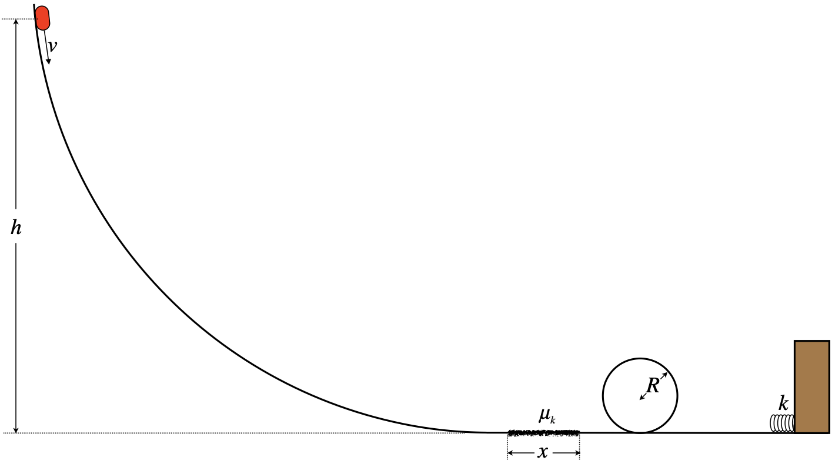
A ball is launched straight up into the air with the apparatus shown below. The ball is pushed upward so that it compresses the spring, and is released from rest. It then travels around a frictionless half-circle track, at the bottom of which is a scale that measures the contact force the ball exerts on the track at that point.
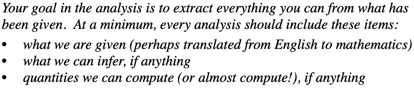
- Analysis
-
The first thing we note here is that if we ignore air resistance, there are no non-conservative forces present, which means that ΔEthermal=0, and the mechanical energy of the system doesn't change from one moment to the next:
KEbefore+Ubefore=KEafter+Uafter
Next, we can see that at various times in the motion of the ball, there are two different potential energies possible - one from the spring and one from gravity. We are told that the ball is launched by the spring, which means that the spring must have been compressed. If we call this amount of compression Δy, then at the moment the ball is released, the system contains an amount of spring potential energy equal to:
Ubefore(spring)=12kΔy2
Determining the amount of gravitational potential energy stored in the system requires that we define a point of zero potential energy. Naturally we can choose anywhere we like as this zero-point, because ultimately only the change in the gravitational potential energy from "before" to "after" will matter, and that will be the same wherever we happen to call Ugrav=0. The diagram labels a height for the ball when it stops rising measured from the bottom of the track, so let's choose that position as zero gravity. Doing this, we can determine the gravitational potential energy of the ball just as it is launched. It's height above the bottom of the track is the radius of the track plus the amount the spring is compressed, so we have:
Ubefore(gravity)=mg(R+Δy)
Clearly the ball starts at rest, so it starts with zero kinetic energy. This completes a "before" picture that we can use to solve a problem. There are a number of "after" times we might be asked about, most of them presumably after the ball has left contact with the spring. At such times, the ball will have a new height and a new speed. The resulting gravitational potential energy and kinetic energy can then be put into the "after" side of the equation, and one can then solve for unknowns.
One item that we have not accounted for is the presence of the scale. It doesn't contribute to the energy of the ball in any way, so why is it even mentioned? Well, the scale provides a clever way to measure the speed of the ball (and therefore its kinetic energy) at the bottom of the track. When the ball passes directly above the scale, it is moving in a circle, and the force exerted by the track on the ball at that point (which is measured by the scale) is straight up toward the center of the circle. The gravity force is straight down, so the net force on the ball is toward the center of the circle, which means its acceleration is centripetal. We therefore have:
Fscale−mg=mv2bottomR
So if we have the scale measurement (and obviously the mass of the ball), we can compute the kinetic energy of the ball at that bottom point from the radius of the track.
A puck slides down a frictionless track, over a short horizontal rough (frictional) patch, around a frictionless loop-de-loop, and into an ideal spring fixed to a wall, where it bounces off and goes back the other way, returning through the loop-de-loop, over the rough patch, and back up the ramp.
- Analysis
-
We clearly have several modes for energy to change form here. The puck will change gravitational potential energy as if moves vertically, it will convert energy from mechanical to thermal when it experiences kinetic friction on the rough patch, potential energy in the spring will change when the puck compresses it, and of course the kinetic energy of the puck can change throughout.
The only weird part here is the loop-de-loop. Like the ramp, it introduces an opportunity for the gravitational potential energy to change, but what else can we say about it? Well, in a previous 'Analyze This' example, we determined a condition for the puck going around the loop to remain in contact. We tend to assume that the puck will make it around the loop to get to the spring, but in fact it has to have at least enough speed at the top of the loop so that it the gravitational force is barely enough to maintain centripetal acceleration. In particular, we found that the minimum speed it must have at the top of the loop is:
vmin=√gR
We can express this as a minimum kinetic energy that the puck must have at the top of the loop in order to maintain contact:
KEmin=12mv2min=12mgR
Given that the gravitational potential energy at the top of the loop is greater than at the bottom by an amount mgΔy=2mgR, it means that to make it around the loop the puck must have a kinetic energy of at least 52mgR. If it came down the ramp from rest with a vertical drop of \(\frac{5}{2}R\), then that would be just enough to let it get around, but of course in this case, the starting point would need to be higher, since the puck loses some of it's kinetic energy to thermal energy thanks to work done by kinetic friction, which we address next.
If we know the coefficient of kinetic friction, then all we need is the normal force between the puck and the rough patch to get the force of kinetic friction, and as this force is constant, the work done by the kinetic friction force is easy to compute, and this energy goes into increasing the thermal energy of the system:
ΔEthermal=−Wf=−∫→Ff⋅→dl=Ffx=μkNx=μkmgx
[The last equality comes from the fact that the surface where the rough patch lies is horizontal, so the normal force equals the puck's weight.]
There is one last important point to make in this analysis. As many places as are available for energy to turn forms, it is not usually necessary to include all of them in the process of solving a problem. Here's an example... Suppose we want to know how high the puck goes back up the ramp after it bounces back one time. We could track its motions through the process, going around the loop and bouncing off the spring, but assuming we know that it has enough energy to traverse the loop-de-loop (something we will need to check, using the criterion found above), we simply set the "before" time as the moment the puck is released and the "after" time when it comes to rest, then all we need to do is include the thermal energy resulting from two trips across the rough patch:
KEbefore+Ubefore=KEafter+Uafter+ΔEthermal⇒0+mgybefore=0+mgyafter+2μkmgx⇒y=h−2μkx
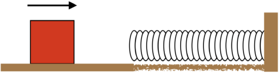
A block slides along a horizontal frictionless surface until it runs into a spring at its equilibrium length. Just as it starts to compress the spring, the surface becomes rough.
- Analysis
-
With everything occurring on a horizontal surface, gravitational potential energy does not play a role. It's not that it isn't present, but it never changes, so it will not appear in our equations. The block will change kinetic energy, and the spring will gain potential energy as it is compressed. In addition, as the spring is being compressed, there is work being done by the kinetic friction force, so this will result in a change of thermal energy for the system. Our energy accounting therefore comes to:
0=ΔKE+ΔUspring+ΔEthermal
If we assume the friction force remains constant along the rough portion of the horizontal surface, then the work done by the constant kinetic friction force is just the negative of that force multiplied by the distance of the slide across the surface. The surface is horizontal, so the normal force equals the weight of the block. This distance is also the compression of the spring, so putting it all together, we have:
ΔEthermal=−Wf=−(−FfΔx)=μkNΔx=μkmgΔx⇒0=12m(v2f−v2o)+(12kΔx2−0)+μkmgΔx
If the roughness of the surface (measured by the coefficient of kinetic friction) does not remain constant along the slide of the block, then the problem becomes a bit tougher. The normal force is the same, but μk is now a function of position, complicating the work integral:
ΔEthermal=−Wf=Δx∫0Ffdx=Δx∫0μ(x)Ndx=mgΔx∫0μ(x)dx