
2.1: Potential Energy of Charge Assembly


- Last updated
- Nov 8, 2022
- Save as PDF

( \newcommand{\kernel}{\mathrm{null}\,}\)
Potential Energy of a Point Charge in a Field
In our brief discussion of the potential energy of dipoles in external fields in Section 1.4, we noted that an electric charge that is displaced within an electric field can have work done on it by the electric force, and this can be expressed as the negative of a change in electrical potential energy. Pruning-down Figure 1.4.5 to a single electric charge, we have:
Figure 2.1.1 – Change of Potential Energy for a Charge Displaced Within a Field
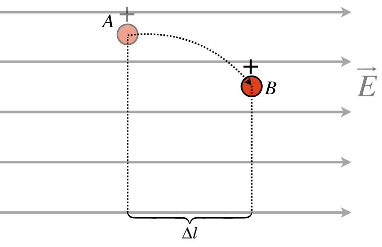
WA→B=B∫A→F⋅→dl=B∫A(qEˆi)⋅(dxˆi+dyˆj)=B∫AqEdx=qEΔl⇒ΔU=UB−UA=−WA→B=−qEΔl
This was easy enough to compute, since the electric field was uniform. We now look at cases where this is not the case. The simplest such case is changing the separation of two point charges. And since starting with point charges is always the basis for more general cases, this is the perfect place to start.
Potential Energy of a Multiple Point Charges
Consider two point charges, q1 and q2 that are separated by an initial distance rA and are moved to a new separation rB (we will assume that only q2 moves). We seek the work done on q2 during this move by the electric field coming from q1, from which we can obtain the change in the system's potential energy.
Figure 2.1.1 – Change of Potential Energy for a Two Point Charges
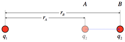
The force between these charges changes as q2 is moved, which means that the work calculation requires a far less trivial integral than was performed for the case of a uniform field. Start by setting up the work integral with the coluomb force:
→Fonq2=q1q24πϵor2ˆr⇒WA→B=B∫A→F⋅→dl=B∫A(q1q24πϵor2ˆr)⋅→dl
The displacement is parallel to the radial unit vector (if it wasn't, the dot product would require that we only take the displacement in that direction anyway), so the product ˆr⋅→dl can be written simply as +dr. Putting this into the integral gives:
WA→B=q1q24πϵorB∫rA1r2dr=q1q24πϵo[1rA−1rB]
The change in potential energy for this process is therefore:
ΔU=−WA→B=q1q24πϵo[1rB−1rA]
As we recall from our study of mechanics, it is only the change in potential energy that matters, but we also find it useful to define a state of zero potential, from which we can reference other states. It is common (though not universal, as well will see later) to reference our point of zero electrostatic potential energy at r=∞. Another way to look at this is to think of the potential energy of a configuration of charges (in this case, two point charges) as the work done in moving the charges from infinite separation to their current proximity. That gives us the following potential energy of two point charges separated by a distance r:
U(r)=−W∞→r=q1q24πϵor
It should be noted that this potential energy is positive if the two charges have the same sign, and negative if they have different signs. This makes sense, since we have to add external work to the system to push the repelling charges together, while attracting charges "want" to come together, which is a characteristic of decreasing potential energy (because the force causes them to speed up, so the loss of potential energy results in a increase of kinetic energy).
When we collect more than just two point charges, we have to account for the potential energy contribution of every pair of charges. This begins to add up when the number of point charges grows. Representing the separation of charge 1 from charge 2 with "r12", charge 1 from charge 3 with "r13," and so on, the total potential energy for a collection of point charges is the sum of all the pairwise contributions:
Utotal=q1q24πϵor12+q1q34πϵor13+q2q34πϵor23…
Example 2.1.1
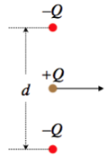
A point charge Q is moving horizontally halfway between two other point charges that are equal in magnitude but opposite in sign, and are held fixed in place. The two negative point charges are separated by a distance d. The positive point charge obviously experiences no net vertical force, so it continues moving horizontally. Find the amount of KE gained or lost (indicate which) by the moving charge at the moment when the three charges form an equilateral triangle.
- Solution
-
The mechanical energy will be conserved, so the change in kinetic energy will equal the negative the change of potential energy. The potential energy in the system that results from the two negative charges interacting with each other never changes (they are held in place), and the potential energy change between the moving charge each of the stationary charges is the same due to symmetry. So all we need to calculate is the change in potential energy between the moving charge and one of the others, and multiply it by two. They are initially separated by a distance d2, and afterward are separated by d, so:
ΔKE=−ΔUsystem=−2[−Q24πϵod−−Q24πϵod2]=−Q22πϵod
The change in kinetic energy is negative, indicating that the charge slows down. This makes sense, given that it is attracted by the other charges, which pull it in the direction opposite to its motion.
Potential Energy of Continuous Distributions
We are of course not only interested in collections of finite numbers of point charges, but continuous distributions of charge as well. To compute the potential energy stored in collecting a distribution of charge can be tricky business. The idea is to set up an integral of contributions to the potential energy due to the addition of an infinitesimal charge.
The simplest example is the case of a conducting sphere of radius R and a surface charge Q (which, thanks to the sphere being a conductor, is evenly-distributed). To determine the potential energy stored in this system, we consider the incremental energy added to it when the surface of the sphere has some intermediate amount of charge q, and we bring dq from infinity to the surface. The field of the spherical shell of charge is identical to that of an equal amount of charge located at its center (which is easily shown using Gauss's law), so the potential energy change of bringing dq from infinity to its surface is:
dU=qdq4πϵoR
Now we keep collecting charge like this until the total charge equals Q. We started with zero charge on the surface, so the limits of integration are 0 to Q:
Usphericalshell=Q∫0qdq4πϵoR=Q28πϵoR
Naturally the potential energy is positive regardless of the sign of Q, because work needs to be done to push together charges of the same sign, regardless of whether they are positive or negative.
We can do the same for a sphere that is uniformly filled with charge, though the procedure requires a bit more thought. Using the same total charge and radius as above, we begin by noting that the charge density within the sphere:
ρ=QV=Q43πR3=3Q4πR3
Now imagine building the solid sphere from the inside-out, one infinitesimally-thin shell at a time. All the charge on such a shell is the same distance from the center, and sees whatever charge is already present as if it was a point charge at the center. Calling the amount of charge already present q, the gain in potential energy that comes from adding the shell (which contains an infinitesimal amount of charge we'll call dq) is:
dU=qdq4πϵor
Notice that the distance to the center is r, not R. This is because the shells that are added are not yet out to the full sphere's radius. To integrate this, we need everything written in terms of a single variable, and the simplest to use is r, which will vary from 0 to R. The amount of charge within a sphere of radius r is:
q=ρV=ρ(43πr3)=Qr3R3
The amount of infinitesimal charge in a spherical shell is the volume of that shell times the density. The volume of the shell is the surface area times the differential radius, so:
dq=ρdV=ρ(4πr2dr)=3Qr2R3dr
Okay, putting all this together and integrating gives us our answer:
Uuniformsolidsphere=r=R∫r=0qdq4πϵor=r=R∫r=0(Qr3R3)(3Qr2R3dr)4πϵor=3Q24πϵoR6r=R∫r=0r4dr=3Q220πϵoR
Notice that despite having the same amount of charge and the same radius, there is more energy stored in this system than in that of a hollow shell. This makes sense if one imagines taking some of the charge on the surface of the hollow sphere and pushing it into the middle to make the sphere a continuous solid collection of uniform charge. Pushing the same-sign charges closer together involves doing work on the system, which adds potential energy to it.
Example 2.1.2
An insulating sphere of radius R contains a net charge that is non-uniformly-distributed. The charge is distributed in a spherically-symmetric manner, depending only upon the distance r from the center of the sphere, according to:
ρ(r)=ρorR
Find the energy stored in this configuration, in terms of the total charge Q present, and the radius of the sphere.
- Solution
-
We start with a partially-assembled sphere with charge q, which occupies the sphere from the center to a radius r. This much charge can be written in terms of ρo and r:
q=∫ρdV=r∫0ρ(r′)4πr′2dr′=4πρoRr∫0r′3dr′=πρoRr4
We can write the constant ρo in terms of the total charge by integrating the entire sphere:
Q=πρoRR4=πρoR3⇒ρo=QπR3
So we can write the charge in the partially-filled sphere and the infinitesimal charge in the thin shell at the outer radius of the partial sphere in terms of the total charge:
q=Qr4R4,dq=4Qr3R4dr
Now we just have to integrate the potential energy function over the full assembly of charge:
U=r=R∫r=0qdq4πϵor=Q2πϵoR8r=R∫r=0r6dr=Q27πϵoR
This energy is higher than for the same amount of charge all on the surface, but lower than for the uniform distribution. This makes sense, since more of the charge has been pushed close together than the hollow shell, but the density gets smaller as we get closer to the center, so more charge is pushed together in the uniform case.
We have limited ourselves to the energy stored in the assembly of spherical charge distributions, thanks to the high degree of symmetry. But the process for less-symmetric assemblies works pretty much the same way, and we will soon see some additional tools that can help with this.