2.1: Spacetime Diagrams

Graphing Spacetime Events

Up to now, we have been representing the position of a spacetime event relative to the spatial axes of Ann and Bob, while representing time by drawing the axes at different positions, with the set of axes remaining fixed being the coordinate system of the observer from whose perspective we are seeing the event. Here we will represent spacetime events in a more efficient and useful (though perhaps a bit more abstract) manner.

We will stay with simplified situations where all the action occurs along the \(x\)-axis, which means that we have room for something else. Specifically, we will draw the position (along \(x\)-axis), and time axes for an observer in an inertial frame whose perspective we are viewing from. With this construction, a spacetime event is simply a point located in the plane of the two axes, and the coordinate position and coordinate time for the observer we are viewing from can be read off the axes directly.

In 9HA we worked with 1-dimensional graphs with the position represented on the vertical axis, and the time on the horizontal axis. In relativity, it is standard (perhaps just to alert the reader to the fact that relativity is being considered) to use time as the vertical axis. What is more, these diagrams give both axes the same units by scaling the vertical axis by the speed of light, \(c\). The resulting representation of spacetime events is called a spacetime or Minkowski diagram.

Figure 2.1.1 – Spacetime Events on a Minkowski Diagram

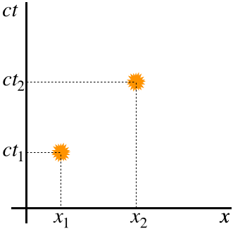
The times indicated by the values on the vertical axis are those measured by synchronized clocks in the frame of the observer represented by these axes. If the two events happen to be aligned vertically, then the two events occur at the same position in this frame, which means the difference \(t_2 - t_1\) in that case is also the proper time interval \(\Delta\tau\). The spacetime interval is related to the "distance" separating these events in the diagram.  If the spacetime interval is measured in an inertial frame, then it is the "length" of the straight line connecting the events, otherwise it is the "arclength" of the curve connecting the events.  All of these quoted words must be very confusing at the moment, but things will be made clearer below.

World Lines

While it is nice to be able to draw two separate events on the same diagram, rather than drawing multiple drawings as we did before, there is an even greater advantage to the tool of the Minkowski diagram – we can represent spacetime trajectories, also known as world lines. Suppose we track a flashing beacon as it moves along the \(x\)-axis. Each flash records a spacetime event with the position it is located and the time of the flash, so we get a string of several points on the spacetime diagram. If the flashing frequency is increased to infinity, then the spacetime points form a continuous curve that tracks the spacetime history of the moving object.

Let's consider a few special world lines. When someone observes a stationary object, its trajectory in the Minkowski diagram must be such that the position doesn't change (but of course the time does). If this person witnesses an object moving at a constant speed, then the world line is sloped, positively when the motion is in the \(+x\) direction, and negatively when the motion is in the \(-x\) direction.

Figure 2.1.2 – Some Simple World Lines

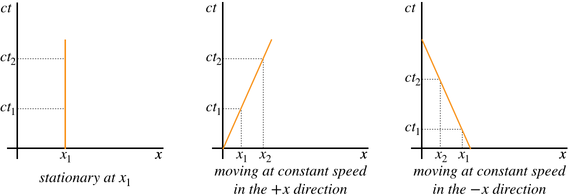
A closer look at the values of the slope of a world line reveals that it is:

\[\text{slope of a world line}=\dfrac{ct_2-ct_1}{x_2-x_1} = \dfrac{c}{u}\;,\;\;\;u\equiv\dfrac{\Delta x}{\Delta t} = \text{speed of the object measured by observer} \]

That is, the inverse of the slope of the world line of an object is the fraction of the speed of light that the observer measures for that object, with the sign representing the direction of motion. If the "object" happens to be a light beam, then its slope is \(\pm 1\).

Example \(\PageIndex{1}\)

Let's return to the thought experiment for the twin paradox involving Ann, Bob, and Chu at the end of Section 1.4, and use a spacetime diagram to depict the race.

1. Draw a spacetime diagram in Ann's reference frame depicting the world lines of both Bob and Chu, and label the important spacetime events along these worldlines.
2. Use the diagram to determine the time on Ann's clock in her spaceship (not at the lattice point in her reference frame) when she sees through her telescope that Chu has changed speed.
3. Use the diagram to determine the time on Bob's clock in his spaceship when he sees through the window of his spaceship that Chu has changed speed.

Solution

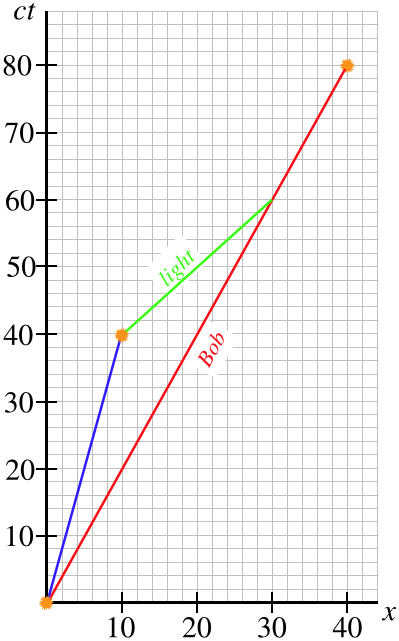
a. The diagram below has light minutes as units on both axes. Both start the race at the same point in spacetime (\(x=0,\;t=0\) in Ann's frame), and end at the same point in spacetime (\(x=40\) light-minutes, \(80\) minutes later). Chu changes speed at \(x=10\) light-minutes, after \(t=40\) minutes. Bob moves at a constant speed of half the speed of light, so the slope of his world line is \(2\). Chu moves at one-quarter the speed of light and then three-quarters the speed of light, so the slopes of his world line segments are \(4\) and \(\frac{4}{3}\), respectively.

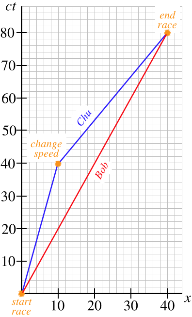
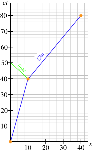
b. Ann doesn't see the event of Chu changing speed until light from that event reaches her. The world line of this light has a slope of \(-1\) because it is coming back to Ann (in the \(-x\)-direction). Drawing this into the diagram shows that she discovers Chu has changed speeds at time \(t=50\) minutes, because that's when the light world line intersects with Ann's world line (which is the vertical axis, since she starts at her origin and never moves).

c. Now we want to know when Bob sees light from the event of Chu changing speed. This time the light goes in the \(+x\)-direction to get to Bob, so it has a slope of \(+1\). This allows us to find the intersection point of the light world line with Bob's world line, but then deriving from that the time on Bob's clock requires a little more work. The simplest way to get this number is to find what the time is on Ann's clock, then use the time dilation formula to get Bob's time. Looking at the diagram below, we see that the time of this intersection in Ann's frame is \(60\) minutes, which in Bob's frame translates to:

\[t_{Bob} = \dfrac{t_{Ann}}{\gamma_v} = \sqrt{1-0.5^2}\left(60\;minutes\right) \approx 52\;minutes\nonumber\]

 

Minkowski Spacetime

Let's represent on spacetime diagrams a comparison of what Ann sees to what Bob sees when they witness the same object's motion. Specifically, let's say they both observe the same clock, which gives off two light flashes at different times, and records those times. Let's further have the clock remain stationary in Ann's frame between these flashes.

With the clock at rest in Ann's frame, the world line for it looks like the first graph in the figure above. With Bob moving in the \(+x\)-direction relative to Ann at a speed \(v\), he sees this same object moving in the \(–x\)-direction at a speed \(v\), which means the worldline he sketches for the object looks like the third graph in the figure above.

As we showed above, the spacetime interval between the two events is the square of the length of the segment of the world line connecting the two events in Ann's spacetime diagram. When we first discussed the nature of time, we made a point of noting that all proper times, and therefore the spacetime interval, are invariants, which means that everyone measures the same value. This would seem to indicate that if Bob measures the length of the segment of the world line he draws between the two events, he should get the same result. In fact this is true, but as we will see, there is a surprise twist.

We found that the time dilation effect gives the comparison between time intervals to be (Bob is the primed frame here):

\[t'_2 - t'_1 = \gamma_v \left(t_2 - t_1\right)\]

But wait, since \(\gamma_v>1\), this means that \(ct'_2 - ct'_1 > ct_2 - c t_1\), and when we look at the spacetime diagrams for Ann and Bob, we see this means that the vertical change in the graph is greater for Bob than it is for Ann.

Figure 2.1.3 – Comparison of Spacetime Intervals for Ann and Bob

It sure doesn't look like there is any way that Ann and Bob could agree on the length of the spacetime interval between these two events! Now for the twist (and the explanation for why we used the quotes on the words "distance", "length", and "arclength" earlier). Let's go back to the light clock thought experiment from Section 1.2. The distance traveled by the light beam was, according to Ann and Bob:

\[\begin{array}{l} Ann: && c\Delta t = 2L \\ Bob: && c\Delta t' = \sqrt{\left(2L\right)^2+\left(x'_2-x'_1\right)^2} \end{array} \]

Eliminating the \(2L\) from these equations gives:

\[c^2\Delta t^2 = c^2\Delta t'^2 - \Delta x'^2\]

The left side of this result is the spacetime interval squared written in Ann's frame, so with the spacetime interval squared being invariant, the right side of the equation must be how it is written in Bob's frame. This looks very close to the Pythagorean theorem, with the exception that the squares that are added are not all positive. Now we can see how the lengths of the world line segments can actually be equal after all. The horizontal leg of the right triangle in Bob's graph actually contributes a negative amount to the length of the hypotenuse. Clearly we have redefined "length" in this context (which we no longer call length, preferring the word "interval" to avoid confusion), but it is necessary to do so to accommodate the nature of time and the constancy of the speed of light.

We therefore reiterate explicitly what we said about the invariance of the spacetime interval back in Section 1.2:

\[\Delta s'^2 = \Delta s^2 \;\;\;\Rightarrow\;\;\; c^2\Delta t'^2 - \left(\Delta x'^2 + \Delta y'^2 + \Delta z'^2\right)=c^2\Delta t^2 - \left(\Delta x^2 + \Delta y^2 + \Delta z^2\right) \]

Notice this works for the case of Ann and Bob above, since \(\Delta x = 0\) for Ann.

Three Measurements of Time Between Two Events

With the tool of spacetime diagrams and a means for computing intervals between events, we can gain a better understanding of the three versions of time.

Figure 2.1.4 – Three Measurements of Time in Spacetime Diagrams

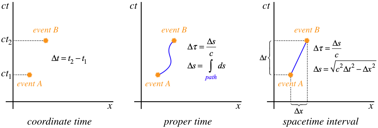
The figure above shows the same two events expressed in the same frame of reference. The first graph shows that the coordinate time elapsed between the two events is simply the difference in the times measured by the synchronized clocks at the two lattice points.

The middle graph expresses a general version of proper time. The time is measured by a clock whose world line passes through both events, and it equals the path length of the clock through spacetime divided by \(c\). This path length is found by doing a line integral to add up all the tiny contributions \(ds\) – each of which is an infinitesimal straight line segment – so:

\[\Delta s = \int\limits_{path} ds = \int\limits_{path} \sqrt{c^2dt^2 - dx^2} \]

The right graph is merely a special case of the middle graph. Integrating \(ds\) to get the path length in that case just gives the length of a straight line (in Minkowski space). Note that the velocity of the clock is changing in the middle graph (the slope of its world line is changing), while in the right graph it is constant. Put another way, the clock is not in an inertial frame in the middle graph, while it is in the right graph.

If a different observer were to graph spacetime coordinate points for the same two events, and then watch the same clocks, the three graphs would look different. The coordinate time separating the two events would change. The world lines of the clock would look different in the other two graphs as well. The world line in the right graph would still be a straight line, but with a different slope. The world line would be different in the middle graph as well, but would still be curved. However, the calculation of \(\Delta s\) in these two graphs would come out the same as they did for the original observer.

Alert

The calculation of \(\Delta s\) for the moving clock in the noninertial frame (middle graph) is the same when computed by any observer. The calculation of \(\Delta s\) for the moving clock in the inertial frame (middle graph) is the same when computed by any observer. Don't confuse this for saying they are the same as each other! The time elapsed on the clock is proportional to the path length \(\Delta s\) through spacetime, and the path length is different for a straight line compared to a curved one.

Here we will repeat something we discussed at the end of Section 1.2, as it may make more sense now that we are armed with the visual aid of the spacetime diagram. We can rewrite Equation 2.1.6 by pulling \(c\;dt\) out of the radical:

\[\Delta s = \int\limits_{path} \sqrt{1 - \frac{1}{c^2}\frac{dx^2}{dt^2}}\;c\;dt = \int \sqrt{1 - \frac{u\left(t\right)^2}{c^2}}\;c\;dt \]

The function \(u\left(t\right)\) is the velocity of the clock as a function of time, which in general can vary during the clock's journey through spacetime. If it does vary, then the radical needs to be kept in the integral. [Naturally "varying velocity" means that such a clock is not remaining in an inertial frame.] If the velocity remains constant, then the radical can be removed from the integral, giving simply:

\[\Delta s = \sqrt{1 - \frac{u^2}{c^2}}c\Delta t \;\;\;\Rightarrow\;\;\; \Delta \tau = \dfrac{\Delta s}{c} = \dfrac{\Delta t}{\gamma_u}\]

We recognize this as the time dilation relationship between the proper time \(\Delta \tau\) in one inertial frame and the coordinate time \(\Delta t\) in an inertial frame moving at a relative speed of \(u\).

We found in our discussion of the twin paradox that the proper time span between two events is longer when measured using an inertial clock than when measured with a non-inertial clock (the twin in the non-inertial space ship ages less over the round trip). In other words, the value of \(\Delta s\) in the middle graph of Figure 2.1.4 is less than the value of \(\Delta s\) in the right graph (remember, the world lines connect the same two events). This seems weird in light of the old adage, "the shortest distance between two points is a straight line," but remember that this is Minkowski space with the weird version of the Pythagorean theorem. To see clearly that this is true, we can change frames to one were the two events are at the same value of \(x\) – remember that these \(\Delta s\) values don't change when we change frames. This will change the right graph such that the world line is a vertical straight line, while the middle graph remains curvy. Because of the \(-dx^2\) contributions to the integral, any horizontal deviations from the vertical path will serve to reduce the magnitude of the integral. So the proper time \(\Delta\tau = \frac{\Delta s}{c}\) for a straight world line between two events (i.e. measured by an inertial clock) is greater than the \(\Delta\tau\) for any non-straight world line between the same two events (i.e. measured by a non-inertial clock).

Example \(\PageIndex{2}\)

Once again returning to the thought experiment for the twin paradox involving Ann, Bob, and Chu at the end of Section 1.4, use the spacetime diagram created in part (a) of Example 2.1.1 above to answer the following:

1. Compute the (Minkowski) length of the world line for Bob to get the time elapsed for him during the race.
2. Repeat the process in part (a) for Chu.

Solution

a. The \(x\) and \(ct\) parts of Bob's world line are \(40\) and \(80\) light-minutes (lm), respectively, so the Minkowski length of his world line is:

\[\Delta s = \sqrt{80^2 - 40^2}\;lm \approx 69 \;lm \nonumber\]

Dividing \(\Delta s\) by the speed of light gives the time, which means that 69 minutes elapse for Bob. This agrees with the result we got in Section 1.4.

b. To compute the length of the world line for Chu, we need to compute the lengths of two separate segments and then add them together.

\[\left. \begin{array}{l} \Delta x_1 = 10\;lm\;,\;\;c\Delta t_1 = 40\;lm && \Rightarrow && \Delta s_1 = \sqrt{40^2-10^2}\;lm \approx 38.7\;lm \\ \Delta x_2 = 30\;lm\;,\;\;c\Delta t_2 = 40\;lm && \Rightarrow && \Delta s_2 = \sqrt{40^2-30^2}\;lm \approx 26.5\;lm \end{array} \right\}\;\;\; \Delta \tau_{Chu} = \dfrac{\Delta s_1 +\Delta s_2}{c} \approx 65min\nonumber\]

Again, this is in agreement with our result before.

Causality

You may have noticed that there is a peculiarity lurking in what we have discussed in this section. In case you haven't, consider the following. We start with events at two points in spacetime, and we want to measure the spacetime interval time that elapses between these events. So we start a clock at one of the events, and move it at a constant speed to the other, recording the times of each event. Combining Equation 2.1.1 with Equation 2.1.6, we see that the clock must record this time span (omitting the \(\Delta y^2\) and \(\Delta z^2\) terms):

\[\Delta \tau = \dfrac{\Delta s}{c} = \dfrac{\sqrt{c^2\Delta t^2-\Delta x^2}}{c} \]

Naturally these two events can occur anywhere in spacetime, so the question is this: If the position in spacetime is such that \(\Delta x^2>c^2\Delta t^2\), exactly what time does the clock measure?! Does an imaginary '\(i\)' suddenly appear in the digital readout?

When we say that a clock cannot be moved from one event to another to record the proper time between the events, what we are really saying is that there is no world-line that connects them. When we think about a spacetime diagram, this means that we can place individual events wherever we like, but we can only connect them with world lines if such a line has a slope whose absolute value is greater than 1 (a speed smaller than \(c\)). This leads to three different categories for how two spacetime events relate to each other:

time-like separation: \(\Delta s^2 > 0\)

This is the case we have been talking about before now, where an object can follow a world line and connect the two events. There is a well-defined proper time associated with the spacetime interval. When two events are separated in this way, we can always find an inertial frame where the events occur at the same spatial position.

light-like separation: \(\Delta s^2 = 0\)

In this case, the world line that connects the two events must belong to a light beam. It isn't possible to change the reference frame to one that is moving at the speed of light relative to another, so although there is a world line that can connect them, it can't belong to a clock.

space-like separation: \(\Delta s^2 < 0\)

For this case, not even light can connect the two events with a world line. If we imagine an event occurring because someone at the spatial position of the event pushes a button to cause a light to flash, then the people responsible for two events separated in this way have no idea that the other event exists, as there is no world line to carry a message about one event to the other event.

This last point about space-like separated events brings up an important concept – that of causality. The study of physics is all about cause-and-effect – it is a net force that causes an acceleration, for example. We see now that we can relate two events according to whether one can cause the other. If there is no way, even in principle, for a message to get from one event to another, then there is no way for the first event to cause the other.

We can characterize what events can be causally-related nicely by using a spacetime diagram. Start by choosing a spacetime event. Then note that to be causally-related to this event, a second event must be positioned such that a straight world line drawn between the two has a slope that is no less than 1 (and if it has a slope of 1, they must be related through a signal that moves at the speed of light). This limits the region of the second event relative to the first into what is called the light cone of that first event.

Figure 2.1.5 – Light Cone of an Event

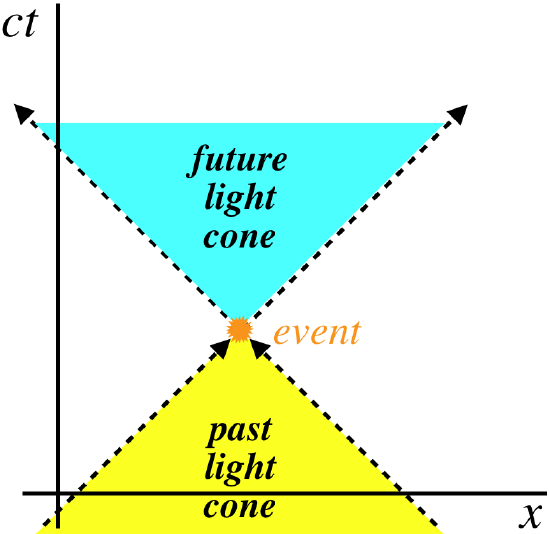
The light cone divides into two halves, called the future and past light cones. Only events in the past light cone can be a cause for the event at the vertex of the light cone, and the event at the vertex of the light cone can only be a cause for events within the future light cone.

It is important to keep in mind that a spacetime diagram is based on a specific frame of reference, and if we change to another frame, the relative positions of the events change (see Figure 2.1.3, for example). But because the spacetime interval is an invariant, what lies within the future(past) light cone of an event in one inertial frame must lie within the future(past) light cone in all inertial frames. We can put this in a far less abstract way: If in Ann's frame event #1 occurs before event #2, and the two events lie within each other's light cones, then event #1 also occurs before event #2 in Bob's frame, no matter what the relative speed of Ann and Bob may be. This assures that if Ann declares that event #1 has caused event #2, there's no observer that can disagree with this on the grounds that event #2 has occurred first.

For a pair of events that do not lie within a light cone (such as two events that are simultaneous in one frame but at different positions, so that they are horizontally-aligned in the spacetime diagram), then the ordering of events is not necessarily preserved in all frames. To see this, let's return to the ladder-and-barn paradox from Section 1.4.

Suppose the farmer's wife is driving one tractor in the \(+x\) direction while the farmer's daughter is driving another tractor in the \(-x\) direction in an effort to get two ladders into the barn at once (both barn doors are open, and they are coming in from opposite directions. According to the farmer, both ladders can be inside the barn at the same time, because the events at the barn doors are simultaneous in his frame. [They are at different positions, so these two events lie outside the light cone from each other.] The farmer's wife notes that the front of her ladder reaches the back of the barn before the rear of her ladder enters, so she says that the event at the back door occurs before the event at the front door. The farmer's daughter sees the exact opposite – the event at the front door occurs first for her.

There is no way that the farmer's wife can ever claim that the event at the back door causes the event at the front door (even though it comes first), because her daughter would argue that it is impossible for the event that occurs second to cause the event that occurs first. Recall that the fact that a light signal cannot get from the back door event to the front door event is exactly what resolved the paradox of whether both doors can be closed with the ladder inside.