
5.12: Manifolds (Part 2)
- Page ID
- 11278

\( \newcommand{\vecs}[1]{\overset { \scriptstyle \rightharpoonup} {\mathbf{#1}} } \)
\( \newcommand{\vecd}[1]{\overset{-\!-\!\rightharpoonup}{\vphantom{a}\smash {#1}}} \)
\( \newcommand{\dsum}{\displaystyle\sum\limits} \)
\( \newcommand{\dint}{\displaystyle\int\limits} \)
\( \newcommand{\dlim}{\displaystyle\lim\limits} \)
\( \newcommand{\id}{\mathrm{id}}\) \( \newcommand{\Span}{\mathrm{span}}\)
( \newcommand{\kernel}{\mathrm{null}\,}\) \( \newcommand{\range}{\mathrm{range}\,}\)
\( \newcommand{\RealPart}{\mathrm{Re}}\) \( \newcommand{\ImaginaryPart}{\mathrm{Im}}\)
\( \newcommand{\Argument}{\mathrm{Arg}}\) \( \newcommand{\norm}[1]{\| #1 \|}\)
\( \newcommand{\inner}[2]{\langle #1, #2 \rangle}\)
\( \newcommand{\Span}{\mathrm{span}}\)
\( \newcommand{\id}{\mathrm{id}}\)
\( \newcommand{\Span}{\mathrm{span}}\)
\( \newcommand{\kernel}{\mathrm{null}\,}\)
\( \newcommand{\range}{\mathrm{range}\,}\)
\( \newcommand{\RealPart}{\mathrm{Re}}\)
\( \newcommand{\ImaginaryPart}{\mathrm{Im}}\)
\( \newcommand{\Argument}{\mathrm{Arg}}\)
\( \newcommand{\norm}[1]{\| #1 \|}\)
\( \newcommand{\inner}[2]{\langle #1, #2 \rangle}\)
\( \newcommand{\Span}{\mathrm{span}}\) \( \newcommand{\AA}{\unicode[.8,0]{x212B}}\)
\( \newcommand{\vectorA}[1]{\vec{#1}} % arrow\)
\( \newcommand{\vectorAt}[1]{\vec{\text{#1}}} % arrow\)
\( \newcommand{\vectorB}[1]{\overset { \scriptstyle \rightharpoonup} {\mathbf{#1}} } \)
\( \newcommand{\vectorC}[1]{\textbf{#1}} \)
\( \newcommand{\vectorD}[1]{\overrightarrow{#1}} \)
\( \newcommand{\vectorDt}[1]{\overrightarrow{\text{#1}}} \)
\( \newcommand{\vectE}[1]{\overset{-\!-\!\rightharpoonup}{\vphantom{a}\smash{\mathbf {#1}}}} \)
\( \newcommand{\vecs}[1]{\overset { \scriptstyle \rightharpoonup} {\mathbf{#1}} } \)
\(\newcommand{\longvect}{\overrightarrow}\)
\( \newcommand{\vecd}[1]{\overset{-\!-\!\rightharpoonup}{\vphantom{a}\smash {#1}}} \)
\(\newcommand{\avec}{\mathbf a}\) \(\newcommand{\bvec}{\mathbf b}\) \(\newcommand{\cvec}{\mathbf c}\) \(\newcommand{\dvec}{\mathbf d}\) \(\newcommand{\dtil}{\widetilde{\mathbf d}}\) \(\newcommand{\evec}{\mathbf e}\) \(\newcommand{\fvec}{\mathbf f}\) \(\newcommand{\nvec}{\mathbf n}\) \(\newcommand{\pvec}{\mathbf p}\) \(\newcommand{\qvec}{\mathbf q}\) \(\newcommand{\svec}{\mathbf s}\) \(\newcommand{\tvec}{\mathbf t}\) \(\newcommand{\uvec}{\mathbf u}\) \(\newcommand{\vvec}{\mathbf v}\) \(\newcommand{\wvec}{\mathbf w}\) \(\newcommand{\xvec}{\mathbf x}\) \(\newcommand{\yvec}{\mathbf y}\) \(\newcommand{\zvec}{\mathbf z}\) \(\newcommand{\rvec}{\mathbf r}\) \(\newcommand{\mvec}{\mathbf m}\) \(\newcommand{\zerovec}{\mathbf 0}\) \(\newcommand{\onevec}{\mathbf 1}\) \(\newcommand{\real}{\mathbb R}\) \(\newcommand{\twovec}[2]{\left[\begin{array}{r}#1 \\ #2 \end{array}\right]}\) \(\newcommand{\ctwovec}[2]{\left[\begin{array}{c}#1 \\ #2 \end{array}\right]}\) \(\newcommand{\threevec}[3]{\left[\begin{array}{r}#1 \\ #2 \\ #3 \end{array}\right]}\) \(\newcommand{\cthreevec}[3]{\left[\begin{array}{c}#1 \\ #2 \\ #3 \end{array}\right]}\) \(\newcommand{\fourvec}[4]{\left[\begin{array}{r}#1 \\ #2 \\ #3 \\ #4 \end{array}\right]}\) \(\newcommand{\cfourvec}[4]{\left[\begin{array}{c}#1 \\ #2 \\ #3 \\ #4 \end{array}\right]}\) \(\newcommand{\fivevec}[5]{\left[\begin{array}{r}#1 \\ #2 \\ #3 \\ #4 \\ #5 \\ \end{array}\right]}\) \(\newcommand{\cfivevec}[5]{\left[\begin{array}{c}#1 \\ #2 \\ #3 \\ #4 \\ #5 \\ \end{array}\right]}\) \(\newcommand{\mattwo}[4]{\left[\begin{array}{rr}#1 \amp #2 \\ #3 \amp #4 \\ \end{array}\right]}\) \(\newcommand{\laspan}[1]{\text{Span}\{#1\}}\) \(\newcommand{\bcal}{\cal B}\) \(\newcommand{\ccal}{\cal C}\) \(\newcommand{\scal}{\cal S}\) \(\newcommand{\wcal}{\cal W}\) \(\newcommand{\ecal}{\cal E}\) \(\newcommand{\coords}[2]{\left\{#1\right\}_{#2}}\) \(\newcommand{\gray}[1]{\color{gray}{#1}}\) \(\newcommand{\lgray}[1]{\color{lightgray}{#1}}\) \(\newcommand{\rank}{\operatorname{rank}}\) \(\newcommand{\row}{\text{Row}}\) \(\newcommand{\col}{\text{Col}}\) \(\renewcommand{\row}{\text{Row}}\) \(\newcommand{\nul}{\text{Nul}}\) \(\newcommand{\var}{\text{Var}}\) \(\newcommand{\corr}{\text{corr}}\) \(\newcommand{\len}[1]{\left|#1\right|}\) \(\newcommand{\bbar}{\overline{\bvec}}\) \(\newcommand{\bhat}{\widehat{\bvec}}\) \(\newcommand{\bperp}{\bvec^\perp}\) \(\newcommand{\xhat}{\widehat{\xvec}}\) \(\newcommand{\vhat}{\widehat{\vvec}}\) \(\newcommand{\uhat}{\widehat{\uvec}}\) \(\newcommand{\what}{\widehat{\wvec}}\) \(\newcommand{\Sighat}{\widehat{\Sigma}}\) \(\newcommand{\lt}{<}\) \(\newcommand{\gt}{>}\) \(\newcommand{\amp}{&}\) \(\definecolor{fillinmathshade}{gray}{0.9}\)Local-coordinate Definition of a Manifold
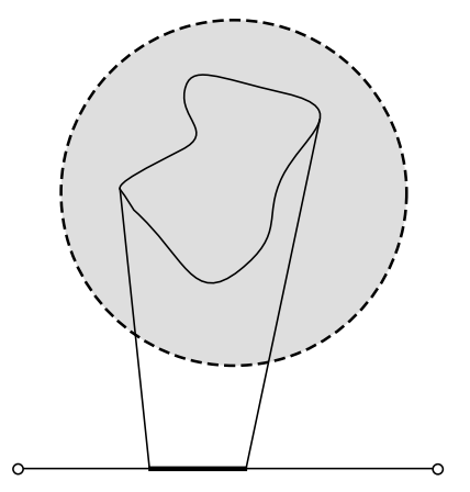
An alternative way of characterizing an n-manifold is as an object that can locally be described by n real coordinates. That is, any sufficiently small neighborhood is homeomorphic to an open set in the space of real-valued n-tuples of the form (x1, x2, . . . , xn). For example, a closed half-plane is not a 2-manifold because no neighborhood of a point on its edge is homeomorphic to any open set in the Cartesian plane.
Exercise \(\PageIndex{1}\)
Self-check: Verify that this alternative definition of a manifold gives the same answers as M1-M3 in all the examples above.
Roughly speaking, the equivalence of the two definitions occurs because we’re using n real numbers as coordinates for the dimensions specified by M1, and the real numbers are the unique number system that has the usual arithmetic operations, is ordered, and is complete in the sense of M3.
As usual when we say that something is “local,” a question arises as to how local is local enough. The language in the definition above about “any sufficiently small neighborhood” is logically akin to the Weierstrass \(\epsilon - \delta\) approach: if Alice gives Bob a manifold and a point on a manifold, Bob can always find some neighborhood around that point that is compatible with coordinates, but it may be an extremely small neighborhood.
Example 20: Coordinates on a circle
If we are to define coordinates on a circle, they should be continuous functions. The angle \(\phi\) about the center therefore doesn’t quite work as a global coordinate, because it has a discontinuity where \(\phi\) = 0 is identified with \(\phi = 2 \pi\). We can get around this by using different coordinates in different regions, as is guaranteed to be possible by the local-coordinate definition of a manifold. For example, we can cover the circle with two open sets, one on the left and one on the right. The left one, L, is defined by deleting only the \(\phi\) = 0 point from the circle. The right one, R, is defined by deleting only the one at \(\phi = \pi\). On L, we use coordinates \(0 < \phi_{L} < 2 \pi\), which are always a continuous function from L to the real numbers. On R, we use \(− \pi < \phi_{R} < \pi\).
In examples like this one, the sets like L and R are referred to as patches. We require that the coordinate maps on the different patches match up smoothly. In this example, we would like all four of the following functions, known as transition maps, to be continuous:
- \(\phi_{L}\) as a function of \(\phi_{R}\) on the domain \(0 < \phi_{R} < \pi\)
- \(\phi_{L}\) as a function of \(\phi_{R}\) on the domain \(− \pi < \phi_{R} < 0\)
- \(\phi_{R}\) as a function of \(\phi_{L}\) on the domain \(0 < \phi_{L} < \pi\)
- \(\phi_{R}\) as a function of \(\phi_{L}\)L on the domain \(\pi < \phi_{L} < 2 \pi\)
The local-coordinate definition only states that a manifold can be coordinatized. That is, the functions that define the coordinate maps are not part of the definition of the manifold, so, for example, if two people define coordinates patches on the unit circle in different ways, they are still talking about exactly the same manifold.
Example 21: Open line segment homeomorphic to a line
Let L be an open line segment, such as the open interval (0, 1). L is homeomorphic to a line, because we can map (0, 1) to the real line through the function f(x) = tan(\(\pi x − \frac{\pi}{2}\)).
Example 22: Closed line segment not homeomorphic to a line
A closed line segment (which is not a manifold) is not homeomorphic to a line. If we map it to a line, then the endpoints have to go to two special points A and B. There is then no way for the mapping to visit the points exterior to the interval [A, B] without visiting A and B more than once.
Example 23: Open line segment not homeomorphic to the interior of a circle
If the interior of a circle could be mapped by a homeomorphism f to an open line segment, then consider what would happen if we took a closed curve lying inside the circle and found its image. By the intermediate value theorem, f would not be one-to-one, but this is a contradiction since f was assumed to be a homeomorphism. This is an example of a more general fact that homeomorphism preserves the dimensionality of a manifold.
Differentiable Manifolds
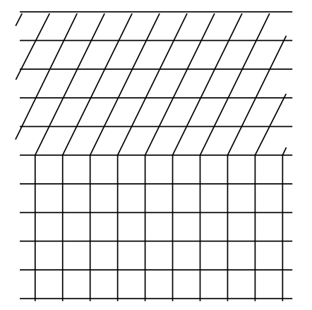
A differentiable manifold means a manifold with enough extra structure so you can do calculus on it, but this extra structure doesn’t necessarily include anything as fancy as a metric. As a concrete example, suppose that in a 1 + 1-dimensional Galilean universe, observer Alice constructs a global coordinate system (t, x). Her spacetime is clearly a manifold, based on the local-coordinate definition, and this is true even though Galilean spacetime doesn’t have a metric. Meanwhile, observer Bob constructs his own coordinate system (t', x'). But something disturbing happens when Alice constructs the transition map from Bob’s coordinate grid to hers. As shown in figure f, Bob’s grid has a kink in it. “Bob,” says Alice, “something is wrong with your coordinate system. I hypothesize that at a certain time, which we can call t = 0, an invisible giant struck your body with an invisible croquet mallet and suddenly changed your state of motion.” “No way, Alice,” Bob answers. “I didn’t feel anything happen at t = 0. I think you’re the one who got whacked.”
By a differentiable manifold we mean one in which this sort of controversy never happens. The manifold comes with an a collection of local coordinate systems, called charts, and wherever these charts overlap, the transition map is differentiable. Every coordinate is a differentiable function of every other coordinate. In fact, we will assume for convenience that not just the first derivative but derivatives of all orders are defined. This makes our manifold not just a differentiable manifold but a smooth manifold. This definition sounds coordinate-dependent, but it isn’t. Our collection of charts (called an atlas) can contain infinitely many possible coordinate systems; we can even specify that it contains all possible coordinate systems that could be obtained from one another by any diffeomorphism.
The Tangent Space
We now formalize the intuitive notion of a tangent vector (section 3.1), following Nowik and Katz.19 Let M be an n-dimensional smooth manifold, so that locally it looks like Euclidean space, describable by real-number coordinates x, y, . . .We now enhance M to form a new topological space, in which the coordinates can include not only real numbers, but numbers that differ infinitesimally from reals, as outlined in example 3. From now on when we say things like “the manifold,” we mean this enhanced version.20 Fix some infinitesimal number \(\epsilon\) for once and for all, and define the notation x = O(\(\epsilon\)) to mean that \(\frac{x}{\epsilon}\) is not infinite.21
Note
It is possible to define a different and larger enhancement, called ∗M, that would include points with infinitely large coordinates. For example, suppose we have a coordinate patch with bounds on the coordinates that can be written down using inequalities, t > 0, 0 ≤ \(\theta\) ≤ \(\frac{\pi}{4}\), . . . Then ∗M would contain any finite, infinitesimal, and infinite values of (t, \(\theta\), . . .) satisfying these inequalities, and this would include infinite values of t. We will not do this here, because the inclusion of idealized points at infinity is more useful in relativity if we do it using a different approach, discussed in section 7.3.
Note
An equivalent and manifestly coordinate-independent definition is that for every smooth real function in a neighborhood of the points, the function differs at these points by an amount that is O(\(\epsilon\)).
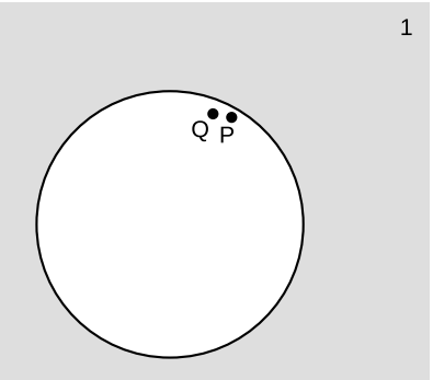
Points in the manifold are considered close if the Euclidean distance between them in coordinate space is O(\(\epsilon\)). This definition sounds coordinate-dependent, but isn’t, and sounds like it’s assuming an actual Euclidean metric, but isn’t.22 Define a prevector at point P as a pair (P,Q) of points that are close, Figure 5.10.7 (1). Define prevectors to be equivalent if the difference between them is infinitesimal even compared to \(\epsilon\).
Definition
A tangent vector at point P is the set of all prevectors at P that are equivalent to a particular prevector at P.
The tangent space TP is the set of all tangent vectors at P. The tangent space has the structure of a vector space over the reals simply by using the coordinate differences to define the vector-space operations, just as we would do if (P, Q) meant an arrow extending from P to Q, as in freshman physics.
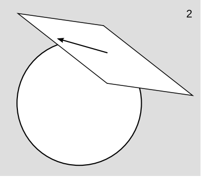
In practice, we don’t really care about the details of the construction of the tangent space, and different people don’t even have to use the same construction. All we care about is that the tangent space has a certain structure. In particular, it has n dimensions, as we would expect intuitively. Since we’re going to forget the details of the construction, it doesn’t matter that we’ve made all tangent vectors infinitesimal by definition. The vector space’s internal structure only has to do with how big the vectors are compared to each other. (If we wanted to, we could scale up all the tangent vectors by a factor of \(\frac{1}{\epsilon}\).) This justifies the visualization in Figure 5.10.7 (2).
Actually it’s not quite true that we only care about the tangent space’s internal structure, because then we could have avoided the fancy definition and simply used the ordinary vector space consisting of n-tuples of real numbers. The fancy definition is needed because it ties the tangent space in a natural way to the structure of the manifold at a particular point. Therefore it will allow us (1) to define parallel transport, which brings a vector from one tangent space to another, and (2) to define components of vectors in a particular coordinate system.
For an alternative definition of the tangent space, see ch. 2 of Carroll.23 Briefly, this involves taking a tangent vector to be something that behaves like a directional derivative. In particular, a partial derivative with respect to a coordinate such as \(\frac{\partial}{\partial x}\) qualifies as a tangent vector, which we think of as pointing in the x direction. The set of such coordinate derivatives forms a basis for the tangent space and gives a convenient way of notating tangent vectors. We will find this notation convenient in section 7.1.
References
19 “Differential geometry via infinitesimal displacements,” arxiv.org/abs/1405.0984
23 Lecture Notes on General Relativity, http://ned.ipac.caltech.edu/level5/March01/Carroll3/Carroll_contents.html.