23.7: Small Oscillations

Any object moving subject to a force associated with a potential energy function that is quadratic will undergo simple harmonic motion,

$$U(x)=U_{0}+\frac{1}{2} k\left(x-x_{e q}\right)^{2} \nonumber$$

where k is a “spring constant”, $x_{e q}$ is the equilibrium position, and the constant $U_{0}$ just depends on the choice of reference point $x_{r e f}$ for zero potential energy, $U\left(x_{r e f}\right)=0$,

$$0=U\left(x_{r e f}\right)=U_{0}+\frac{1}{2} k\left(x_{r e f}-x_{e q}\right)^{2} \nonumber$$

Therefore the constant is

$$U_{0}=-\frac{1}{2} k\left(x_{r e f}-x_{e q}\right)^{2} \nonumber$$

The minimum of the potential $x_{0}$ corresponds to the point where the x -component of the force is zero,

$$\left.\frac{d U}{d x}\right|_{x=x_{0}}=2 k\left(x_{0}-x_{e q}\right)=0 \Rightarrow x_{0}=x_{e q} \nonumber$$

corresponding to the equilibrium position. Therefore the constant is $U\left(x_{0}\right)=U_{0}$ and we rewrite our potential function as

$$U(x)=U\left(x_{0}\right)+\frac{1}{2} k\left(x-x_{0}\right)^{2} \nonumber$$

Now suppose that a potential energy function is not quadratic but still has a minimum at $x_{0}$. For example, consider the potential energy function

$$U(x)=-U_{1}\left(\left(\frac{x}{x_{1}}\right)^{3}-\left(\frac{x}{x_{1}}\right)^{2}\right) \nonumber$$

(Figure 23.22), which has a stable minimum at $x_{0}$,

Figure 23.22 Potential energy function with stable minima and unstable maxima

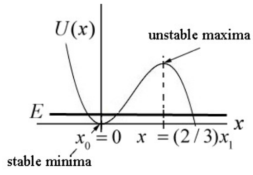
When the energy of the system is very close to the value of the potential energy at the minimum $U\left(x_{0}\right)$, we shall show that the system will undergo small oscillations about the minimum value $x_{0}$. We shall use the Taylor formula to approximate the potential function as a polynomial. We shall show that near the minimum $x_{0}$ we can approximate the potential function by a quadratic function similar to Equation (23.7.5) and show that the system undergoes simple harmonic motion for small oscillations about the minimum $x_{0}$.

We begin by expanding the potential energy function about the minimum point using the Taylor formula

$$U(x)=U\left(x_{0}\right)+\left.\frac{d U}{d x}\right|_{x=x_{0}}\left(x-x_{0}\right)+\left.\frac{1}{2 !} \frac{d^{2} U}{d x^{2}}\right|_{x=x_{0}}\left(x-x_{0}\right)^{2}+\left.\frac{1}{3 !} \frac{d^{3} U}{d x^{3}}\right|_{x=x_{0}}\left(x-x_{0}\right)^{3}+\cdots \nonumber$$

where $\left.\frac{1}{3 !} \frac{d^{3} U}{d x^{3}}\right|_{x=x_{0}}\left(x-x_{0}\right)^{3}$ is a third order term in that it is proportional to $\left(x-x_{0}\right)^{3}$, and $\left.\frac{d^{3} U}{d x^{3}}\right|_{x=x_{0}},\left.\frac{d^{2} U}{d x^{2}}\right|_{x=x_{0}}, \quad \text { and }\left.\frac{d U}{d x}\right|_{x=x_{0}}$ are constants. If $x_{0}$ is the minimum of the potential energy, then the linear term is zero, because

$$\left.\frac{d U}{d x}\right|_{x=x_{0}}=0 \nonumber$$

and so Equation ((23.7.7)) becomes

$$U(x) \simeq U\left(x_{0}\right)+\left.\frac{1}{2} \frac{d^{2} U}{d x^{2}}\right|_{x=x_{0}}\left(x-x_{0}\right)^{2}+\left.\frac{1}{3 !} \frac{d^{3} U}{d x^{3}}\right|_{x=x_{0}}\left(x-x_{0}\right)^{3}+\cdots \nonumber$$

For small displacements from the equilibrium point such that $\left|x-x_{0}\right|$ is sufficiently small, the third order term and higher order terms are very small and can be ignored. Then the potential energy function is approximately a quadratic function,

$$U(x) \simeq U\left(x_{0}\right)+\left.\frac{1}{2} \frac{d^{2} U}{d x^{2}}\right|_{x=x_{0}}\left(x-x_{0}\right)^{2}=U\left(x_{0}\right)+\frac{1}{2} k_{e f f}\left(x-x_{0}\right)^{2} \nonumber$$

where we define $k_{eff}$, the effective spring constant, by

$$\left.k_{e f f} \equiv \frac{d^{2} U}{d x^{2}}\right|_{x=x_{0}} \nonumber$$

Because the potential energy function is now approximated by a quadratic function, the system will undergo simple harmonic motion for small displacements from the minimum with a force given by

$$F_{x}=-\frac{d U}{d x}=-k_{e f f}\left(x-x_{0}\right) \nonumber$$

At $x=x_{0}$, the force is zero

$$F_{x}\left(x_{0}\right)=\frac{d U}{d x}\left(x_{0}\right)=0 \nonumber$$

We can determine the period of oscillation by substituting Equation (23.7.12) into Newton’s Second Law

$$-k_{eff}\left(x-x_{0}\right)=m_{eff} \frac{d^{2} x}{d t^{2}} \nonumber$$

where $m_{eff}$ is the effective mass. For a two-particle system, the effective mass is the reduced mass of the system.

$$m_{eff}=\frac{m_{1} m_{2}}{m_{1}+m_{2}} \equiv \mu_{red} \nonumber$$

Equation (23.7.14) has the same form as the spring-object ideal oscillator. Therefore the angular frequency of small oscillations is given by

$$\omega_{0}=\sqrt{\frac{k_{e f f}}{m_{e f f}}}=\sqrt{(\left.\frac{d^{2} U}{d x^{2}}\right|_{x=x_{0}})/{m_{e f f}}} \nonumber$$

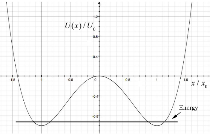
Example 23.6: Quartic Potential

A system with effective mass m has a potential energy given by

$$U(x)=U_{0}\left(-2\left(\frac{x}{x_{0}}\right)^{2}+\left(\frac{x}{x_{0}}\right)^{4}\right) \nonumber$$

where $U_{0}$ and $x_{0}$ are positive constants and $U(0)=0$ (a) Find the points where the force on the particle is zero. Classify these points as stable or unstable. Calculate the value of $U(x) / U_{0}$ at these equilibrium points. (b) If the particle is given a small displacement from an equilibrium point, find the angular frequency of small oscillation.

Solution: (a) A plot of $U(x) / U_{0}$ as a function of $x / x_{0}$ is shown in Figure 23.23.

Figure 22.23 Plot of $U(x) / U_{0}$ as a function of $x / x_{0}$

The force on the particle is zero at the minimum of the potential energy,

$$\begin{array}{l} 0=\frac{d U}{d x}=U_{0}\left(-4\left(\frac{1}{x_{0}}\right)^{2} x+4\left(\frac{1}{x_{0}}\right)^{4} x^{3}\right) \\ =-4 U_{0} x\left(\frac{1}{x_{0}}\right)^{2}\left(1-\left(\frac{x}{x_{0}}\right)^{2}\right) \Rightarrow x^{2}=x_{0}^{2} \text { and } x=0 \end{array} \nonumber$$

The equilibrium points are at $x=\pm x_{0}$ which are stable and x = 0 which is unstable. The second derivative of the potential energy is given by

$$\frac{d^{2} U}{d x^{2}}=U_{0}\left(-4\left(\frac{1}{x_{0}}\right)^{2}+12\left(\frac{1}{x_{0}}\right)^{4} x^{2}\right) \nonumber$$

If the particle is given a small displacement from $x=x_{0}$ then

$$\left.\frac{d^{2} U}{d x^{2}}\right|_{x=x_{0}}=U_{0}\left(-4\left(\frac{1}{x_{0}}\right)^{2}+12\left(\frac{1}{x_{0}}\right)^{4} x_{0}^{2}\right)=U_{0} \frac{8}{x_{0}^{2}} \nonumber$$

(b) The angular frequency of small oscillations is given by

$$\omega_{0}=\sqrt{\left.\frac{d^{2} U}{d x^{2}}\right|_{x=x_{0}} / m}=\sqrt{\frac{8 U_{0}}{m x_{0}^{2}}} \nonumber$$

Example 23.7: Lennard-Jones 6-12 Potential

A commonly used potential energy function to describe the interaction between two atoms is the Lennard-Jones 6-12 potential

$$U(r)=U_{0}\left[\left(r_{0} / r\right)^{12}-2\left(r_{0} / r\right)^{6}\right] ; r>0 \nonumber$$

where r is the distance between the atoms. Find the angular frequency of small oscillations about the stable equilibrium position for two identical atoms bound to each other by the LennardJones interaction. Let m denote the effective mass of the system of two atoms.

Solution: The equilibrium points are found by setting the first derivative of the potential energy equal to zero,

$$0=\frac{d U}{d r}=U_{0}\left[-12 r_{0}^{12} r^{-13}+12 r_{0}^{6} r^{-7}\right]=U_{0} 12 r_{0}^{6} r^{-7}\left[-\left(\frac{r_{0}}{r}\right)^{6}+1\right] \nonumber$$

The equilibrium point occurs when $r=r_{0}$ The second derivative of the potential energy function is

$$\frac{d^{2} U}{d r^{2}}=U_{0}\left[+(12)(13) r_{0}^{12} r^{-14}-(12)(7) r_{0}^{6} r^{-8}\right] \nonumber$$

Evaluating this at $r=r_{0}$ yields

$$\left.\frac{d^{2} U}{d r^{2}}\right|_{r=r_{0}}=72 U_{0} r_{0}^{-2} \nonumber$$

The angular frequency of small oscillation is therefore

$$\omega_{0}=\sqrt{\left.\frac{d^{2} U}{d r^{2}}\right|_{r=r_{0}} / m} \nonumber$$

$$=\sqrt{72 U_{0} / m r_{0}^{2}} \nonumber$$