28.6: Laminar and Turbulent Flow

Introduction

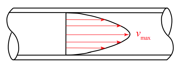
During the flow of a fluid, different layers of the fluid may be flowing at different speeds relative to each other, one layer sliding over another layer. For example consider a fluid flowing in a long cylindrical pipe. For slow velocities, the fluid particles move along lines parallel to the wall. Far from the entrance of the pipe, the flow is steady (fully developed). This steady flow is called laminar flow. The fluid at the wall of the pipe is at rest with respect to the pipe. This is referred to as the no-slip condition and is experimentally holds for all points in which a fluid is in contact with a wall. The speed of the fluid increases towards the interior of the pipe reaching a maximum, v max , at the center. The velocity profile across a cross section of the pipe exhibiting fully developed flow is shown in Figure 28.10. This parabolic velocity profile has a non-zero velocity gradient that is normal to the flow.

Figure 28.10 Steady laminar flow in a pipe with a non-zero velocity gradient

Viscosity

Due to the cylindrical geometry of the pipe, cylindrical layers of fluid are sliding with respect to one another resulting in tangential forces between layers. The tangential force per area is called a shear stress. The viscosity of a fluid is a measure of the resistance to this sliding motion of one layer of the fluid with respect to another layer. A perfect fluid has no tangential forces between layers. A fluid is called Newtonian if the shear forces per unit area are proportional to the velocity gradient. For a Newtonian fluid undergoing laminar flow in the cylindrical pipe, the shear stress, $\sigma_{S}$, is given by

$$\sigma_{s}=\eta \frac{d v}{d r} \nonumber$$

where $\eta$ is the constant of proportionality and is called the absolute viscosity, r is the radial distance form the central axis of the pipe, and $d v / d r$ is the velocity gradient normal to the flow.

The SI units for viscosity are $\text { poise }=10^{-1} \mathrm{Pa} \cdot \mathrm{s}$. Some typical values for viscosity for fluids at specified temperatures are given in Table 1.

Table 1: Coefficients of absolute viscosity

$$\begin{array}{||l|l|} \hline \text { fluid } & \text { Coefficient of absolute viscosity } \eta \\ \hline \text { oil } & 1-10 \text { poise } \\ \hline \text { Water at } 0^{\circ} & 1.79 \times 10^{-2} \text {poise } \\ \hline \text { Water at } 100^{\circ} & 0.28 \times 10^{-2} \text {poise } \\ \hline \text { Air at } 20^{\circ} & 1.81 \times 10^{-4} \text {poise } \\ \hline \end{array} \nonumber$$

At a certain flow rate, this resistance suddenly increases and the fluid particles no longer follow straight lines but appear to move randomly although the average motion is still along the axis of the pipe. This type of flow is called turbulent flow. Osbourne Reynolds was the first to experimentally measure these two types of flow. He was able to characterize the transition between these two types of flow by a parameter called the Reynolds number that depends on the average velocity of the fluid in the pipe, the diameter, and the viscosity of the fluid. The transition point between flows corresponds to a value of the Reynolds number that is associated with a sudden increase in the friction between layers of the fluid. Much after Reynolds initial observations, it was experimentally noted that a small disturbance in the laminar flow could rapidly grow and produce turbulent flow.

Example 28.3 Couette Flow

Consider the flow of a Newtonian fluid between two very long parallel plates, each plate of width $w$, length $s$, and separated by a distance $d$. The upper plate moves with a constant relative speed $v_{0}$ with respect to the lower plate, (Figure 28.11).

Figure 28.11 Laminar flow between two plates moving with relative speed $v_{0}$

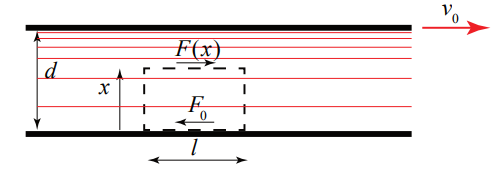
Choose a reference frame in which the lower plate, located on the plane at $x = 0$, is at rest. Choose a volume element of length $l$ and cross sectional area $A$, with one side in contact with the plate at rest, and the other side located a distance $x$ from the lower plate. The velocity gradient in the direction normal to the flow is $d v / d x$. The shear force on the volume element due to the fluid above the element is given by

$$F(x)=\eta A \frac{d v}{d x} \nonumber$$

The shear force is balanced by the shear force $F_{0}$ of the lower plate on the element, such that $F(x)=F_{0}$. Hence

$$F_{0}=\eta A \frac{d v}{d x} \nonumber$$

The velocity of the fluid at the lower plate is zero. The integral version of this differential equation is then

$$\frac{1}{\eta A} \int_{x^{\prime}=0}^{x^{\prime}=x} F_{0} d x^{\prime}=\int_{v^{\prime}=0}^{v^{\prime}=v(x)} d v^{\prime} \nonumber$$

Integration yields

$$\frac{F_{0}}{\eta A} x=v(x) \nonumber$$

The velocity of the fluid at the upper plate is $v_{0}$, therefore the constant shear stress is given by

$$\frac{F_{0}}{A}=\frac{\eta v_{0}}{d} \nonumber$$

hence the velocity profile is

$$v(x)=\frac{v_{0}}{d} x \nonumber$$

This type of flow is known as Couette flow.

Example 28.4 Laminar flow in a cylindrical pipe.

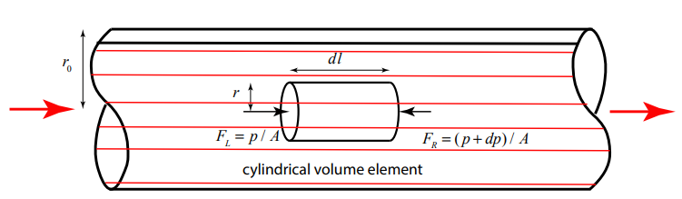
Let’s consider a long cylindrical pipe of radius $r_{0}$ in which the fluid undergoes laminar flow with each fluid particle moves in a line parallel to the pipe axis. Choose a cylindrical volume element of length $dl$ and radius $r$, centered along the pipe axis as shown in Figure 28.12. There is a pressure drop $d p<0$ over the length of the volume element resulting in forces on each end cap. Denote the force on the left end cap by $F_{L}=p / A$ and the force on the right end cap by $F_{R}=(p+d p) / A$ on the right end cap, where $A=\pi r^{2}$ is the cross sectional area of the end cap.

Figure 28.12: Volume element for steady laminar flow in a pipe

The forces on the volume element sum to zero and are due to the pressure difference and the shear stress; hence

$$F_{L}-F_{R}+\sigma_{s} 2 \pi r d l=0 \nonumber$$

Using our Newtonian model for the fluid (Equation (28.4.30) and expressing the force in terms of pressure, Equation (28.4.37) becomes

$$\frac{d p}{2 \eta d l} r=\frac{d v}{d r} \nonumber$$

Equation (28.4.38) can be integrated by the method of separation of variables with boundary conditions $v(r=0)=v_{\max } \text { and } v\left(r=r_{0}\right)=0$. (Recall that for laminar flow of a Newtonian fluid the velocity of a fluid is always zero at the surface of a solid.)

$$\frac{d p}{2 \eta d l} \int_{r^{\prime}=r}^{r^{\prime}=r_{0}} r^{\prime} d r^{\prime}=\int_{v^{\prime}=v(r)}^{v^{\prime}\left(r=r_{0}\right)=0} d v^{\prime} \nonumber$$

Integration then yields

$$v(r)=-\frac{d p}{4 \eta d l}\left(r_{0}^{2}-r^{2}\right) \nonumber$$

Recall that the pressure drop $d p<0$. The maximum velocity at the center is then

$$v_{\max }=v(r=0)=-\frac{d p}{4 \eta d l} r_{0}^{2} \nonumber$$

To determine the flow rate through the pipe, choose a ring of radius $\boldsymbol{r}$ and thickness $\boldsymbol{r}$, oriented normal to the flow. The flow through the ring is then

$$v(r) 2 \pi r d r=-\frac{d p \pi}{2 \eta d l}\left(r_{0}^{2}-r^{2}\right) r d r \nonumber$$

Integrating over the cross sectional area of the pipe yields

$$\begin{array}{l} Q=\int_{r=0}^{r=r_{0}} v(r) 2 \pi r d r \\ Q=-\frac{d p \pi}{2 \eta d l} \int_{r=0}^{r=r_{0}}\left(r_{0}^{2}-r^{2}\right) r d r=-\left.\frac{d p \pi}{2 \eta d l}\left(r_{0}^{2} r^{2} / 2-r^{4} / 4\right)\right|_{r=0} ^{r=r_{0}}=\frac{\pi r_{0}^{4}}{8 \eta d l}|d p| \end{array} \nonumber$$

The average velocity is then

$$v_{\text {ave}}=\frac{Q}{\pi r_{0}^{2}}=-\frac{d p}{8 \eta d l} r_{0}^{2} \nonumber$$

Notice that the pressure difference and the volume flow rate are related by

$$|d p|=\frac{8 \eta d l}{\pi r_{0}^{4}} Q \nonumber$$

which is equal to one half the maximum velocity at the center of the pipe. We can rewrite Equation (28.4.45) in terms of the average velocity as

$$|d p|=\frac{8 \eta d l}{\pi r_{0}^{4}} Q=\frac{64 \eta d l}{v_{a v e} 2 d^{2}} v_{a v e}^{2} \nonumber$$

where $d=2 r_{0}$ is the diameter of the pipe. For a pipe of length $l$ and pressure difference $\Delta p$, the head loss in a pipe is defined as the ratio

$$h_{f}=\frac{|\Delta p|}{\rho g}=\frac{64}{\left(\rho v_{\text {ave}} d / \eta\right)} \frac{v_{\text {me}}^{2}}{2 g} \frac{l}{d} \nonumber$$

where we have extended Equation (28.4.46) for the entire length of the pipe. Head loss is also written in terms of a loss coefficient $k$ according to

$$h_{f}=k \frac{v_{\text {ave}}^{2}}{2 g} \nonumber$$

For a long straight cylindrical pipe, the loss coefficient can be written in terms of a factor $f$ times an equivalent length of the pipe

$$k=f \frac{l}{d} \nonumber$$

The factor $f$ can be determined by comparing Equations (28.4.47)-(28.4.49) yielding

$$f=\frac{64}{\left(\rho v_{\text {ave }} d / \eta\right)}=\frac{64}{\operatorname{Re}} \nonumber$$

where $Re$ is the Reynolds number and is given by

$$\operatorname{Re}=\rho v_{\text {ave }} d / \eta \nonumber$$