4.4: Free Rotation

Now let us proceed to the more complex case when the rotation axis is not fixed. A good illustration of the complexity arising in this case comes from the case of a rigid body left alone, i.e. not subjected to external forces and hence with its potential energy $U$ constant. Since in this case, according to Eq. (44), the center of mass moves (as measured from any inertial reference frame) with a constant velocity, we can always use a convenient inertial reference frame with the origin at that point. From the point of view of such a frame, the body’s motion is a pure rotation, and $T_{\text {tran }}=0$. Hence, the system’s Lagrangian equals just the rotational energy (15), which is, first, a quadratic-homogeneous function of the components $\omega_{j}$ (which may be taken for generalized velocities), and, second, does not depend on time explicitly. As we know from Chapter 2, in this case the mechanical energy, here equal to $T_{\text {rot }}$ alone, is conserved. According to Eq. (15), for the principal-axes components of the vector $\omega$, this means

$$T_{\text {rot }}=\sum_{j=1}^{3} \frac{I_{j}}{2} \omega_{j}^{2}=\text { const }$$ Next, as Eq. (33) shows, in the absence of external forces, the angular momentum $\mathbf{L}$ of the body is conserved as well. However, though we can certainly use Eq. (26) to represent this fact as $$\mathbf{L}=\sum_{j=1}^{3} I_{j} \omega_{j} \mathbf{n}_{j}=\text { const },$$ where $\mathbf{n}_{j}$ are the principal axes, this does not mean that all components $\omega_{j}$ are constant, because the principal axes are fixed relative to the rigid body, and hence may rotate with it.

Before exploring these complications, let us briefly mention two conceptually trivial, but practically very important, particular cases. The first is a spherical top $\left(I_{1}=I_{2}=I_{3}=I\right)$. In this case, Eqs. (55) and (56) imply that all components of the vector $\omega=\mathbf{L} / \mathrm{I}$, i.e. both the magnitude and the direction of the angular velocity are conserved, for any initial spin. In other words, the body conserves its rotation speed and axis direction, as measured in an inertial frame. The most obvious example is a spherical planet. For example, our Mother Earth, rotating about its axis with angular velocity $\omega=2 \pi /(1$ day $) \approx$ $7.3 \times 10^{-5} \mathrm{~s}^{-1}$, keeps its axis at a nearly constant angle of $23^{\circ} 27$ ’ to the ecliptic pole, i.e. the axis normal to the plane of its motion around the Sun. (In Sec. 6 below, we will discuss some very slow motions of this axis, due to gravity effects.)

Spherical tops are also used in the most accurate gyroscopes, usually with gas-jet or magnetic suspension in vacuum. If done carefully, such systems may have spectacular stability. For example, the gyroscope system of the Gravity Probe B satellite experiment, flown in 2004-5, was based on quartz spheres - round with precision of about $10 \mathrm{~nm}$ and covered with superconducting thin films (which enabled their magnetic suspension and monitoring). The whole system was stable enough to measure that the so-called geodetic effect in general relativity (essentially, the space curving by Earth’s mass), resulting in the axis’ precession by only $6.6$ arc seconds per year, i.e. with a precession frequency of just $\sim 10^{-11} \mathrm{~s}^{-1}$, agrees with theory with a record $\sim 0.3 \%$ accuracy. ${ }^{9}$

The second simple case is that of the symmetric top $\left(I_{1}=I_{2} \neq I_{3}\right)$, with the initial vector $\mathbf{L}$ aligned with the main principal axis. In this case, $\omega=\mathbf{L} / \mathrm{I}_{3}=$ const, so that the rotation axis is conserved. ${ }^{10}$ Such tops, typically in the shape of a flywheel (heavy, flat rotor), and supported by a three-ring gimbal system (also called the “Cardan suspensions”) that allow for torque-free rotation about three mutually perpendicular axes,¹¹ are broadly used in more common gyroscopes. Invented by Léon Foucault in the 1850s and made practical by H. Anschütz-Kaempfe, such gyroscopes have become core parts of automatic guidance systems, for example, in ships, airplanes, missiles, etc. Even if its support wobbles and/or drifts, the suspended gyroscope sustains its direction relative to an inertial reference frame.¹²

However, in the general case with no such special initial alignment, the dynamics of symmetric tops is more complicated. In this case, the vector $\mathbf{L}$ is still conserved, including its direction, but the vector $\omega$ is not. Indeed, let us direct the $\mathbf{n}_{2}$ axis normally to the common plane of vectors $\mathbf{L}$ and the current instantaneous direction $\mathbf{n}_{3}$ of the main principal axis (in Figure 8 below, the plane of the drawing); then, in that particular instant, $L_{2}=0$. Now let us recall that in a symmetric top, the axis $\mathbf{n}_{2}$ is a principal one. According to Eq. (26) with $j=2$, the corresponding component $\omega_{2}$ has to be equal to $L_{2} / I_{2}$, so it is equal to zero. This means that the vector $\omega$ lies in this plane (the common plane of vectors $\mathbf{L}$ and $\mathbf{n}_{3}$ ) as well - see Figure 8a.

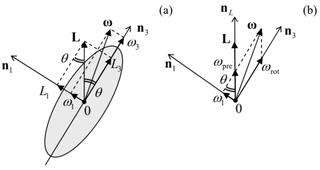Figure 4.8. Free rotation of a symmetric top: (a) the general configuration of vectors, and (b) calculating the free precession frequency.

Now consider any point located on the main principal axis $\mathbf{n}_{3}$, and hence on the plane $\left[\mathbf{n}_{3}, \mathbf{L}\right]$. Since $\omega$ is the instantaneous axis of rotation, according to Eq. (9), the instantaneous velocity $\mathbf{v}=\omega \times \mathbf{r}$ of the point is directed normally to that plane. Since this is true for each point of the main axis (besides only one, with $\mathbf{r}=0$, i.e. the center of mass, which does not move), this axis as a whole has to move perpendicular to the common plane of the vectors $\mathbf{L}, \omega$, and $\mathbf{n}_{3}$. Since this conclusion is valid for any moment of time, it means that the vectors $\omega$ and $\mathbf{n}_{3}$ rotate about the space-fixed vector $\mathbf{L}$ together, with some angular velocity $\omega_{\text {pre }}$, at each moment staying within one plane. This effect is usually called the free precession (or "torque-free", or "regular") precession, and has to be clearly distinguished it from the completely different effect of the torque-induced precession, which will be discussed in the next section.To calculate $\omega_{\text {pre }}$, let us represent the instant vector $\omega$ as a sum of not its Cartesian components (as in Figure 8a), but rather of two non-orthogonal vectors directed along $\mathbf{n}_{3}$ and $\mathbf{L}$ (Figure 8b):

$$\boldsymbol{\omega}=\omega_{\mathrm{rot}} \mathbf{n}_{3}+\omega_{\mathrm{pre}} \mathbf{n}_{L}, \quad \mathbf{n}_{L} \equiv \frac{\mathbf{L}}{L} .$$

Figure 8b shows that $\omega_{\text {rot }}$ has the meaning of the angular velocity of rotation of the body about its main principal axis, while $\omega_{\text {pre }}$ is the angular velocity of rotation of that axis about the constant direction of the vector $\mathbf{L}$, i.e. the frequency of precession, i.e. exactly what we are trying to find. Now $\omega_{\text {pre }}$ may be readily calculated from the comparison of two panels of Figure 8, by noticing that the same angle $\theta$ between the vectors $\mathbf{L}$ and $\mathbf{n}_{3}$ participates in two relations:

$$\sin \theta=\frac{L_{1}}{L}=\frac{\omega_{1}}{\omega_{\text {pre }}} .$$ Since the $\mathbf{n}_{1}$-axis is a principal one, we may use Eq. (26) for $j=1$, i.e. $L_{1}=I_{1} \omega_{1}$, to eliminate $\omega_{1}$ from Eq. (58), and get a very simple formula $$\omega_{\text {pre }}=\frac{L}{I_{1}} .$$ This result shows that the precession frequency is constant and independent of the alignment of the vector $\mathbf{L}$ with the main principal axis $\mathbf{n}_{3}$, while the amplitude of this motion (characterized by the angle $\theta$ ) does depend on the alignment, and vanishes if $\mathbf{L}$ is parallel to $\mathbf{n}_{3} \cdot{ }^{13}$ Note also that if all principal moments of inertia are of the same order, $\omega_{\text {pre }}$ is of the same order as the total angular speed $\omega \equiv|\omega|$ of rotation.

Now let us briefly discuss the free precession in the general case of an "asymmetric top", i.e. a body with arbitrary $I_{1} \neq I_{2} \neq I_{3}$. In this case, the effect is more complex because here not only the direction but also the magnitude of the instantaneous angular velocity $\omega$ may evolve in time. If we are only interested in the relation between the instantaneous values of $\omega_{j}$ and $L_{j}$, i.e. the "trajectories" of the vectors $\omega$ and $\mathbf{L}$ as observed from the reference frame $\left\{\mathbf{n}_{1}, \mathbf{n}_{2}, \mathbf{n}_{3}\right\}$ of the principal axes of the body (rather than the explicit law of their time evolution), they may be found directly from the conservation laws. (Let me emphasize again that the vector $\mathbf{L}$, being constant in an inertial reference frame, generally evolves in the frame rotating with the body.) Indeed, Eq. (55) may be understood as the equation of an ellipsoid in Cartesian coordinates $\left\{\omega_{1}, \omega_{2}, \omega_{3}\right\}$, so that for a free body, the vector $\omega$ has to stay on the surface of that ellipsoid. ${ }^{14}$ On the other hand, since the reference frame rotation preserves the length of any vector, the magnitude (but not the direction!) of the vector $\mathbf{L}$ is also an integral of motion in the moving frame, and we can write

$$L^{2} \equiv \sum_{j=1}^{3} L_{j}^{2}=\sum_{j=1}^{3} I_{j}^{2} \omega_{j}^{2}=\text { const }$$ Hence the trajectory of the vector $\omega$ follows the closed curve formed by the intersection of two ellipsoids, (55) and (60). It is evident that this trajectory is generally "taco-edge-shaped", i.e. more complex than a planar circle, but never very complex either. ${ }^{15}$

The same argument may be repeated for the vector $\mathbf{L}$, for whom the first form of Eq. (60) descries a sphere, and Eq. (55), another ellipsoid:

$$T_{\mathrm{rot}}=\sum_{j=1}^{3} \frac{1}{2 I_{j}} L_{j}^{2}=\mathrm{const} .$$ On the other hand, if we are interested in the trajectory of the vector $\omega$ as observed from an inertial frame (in which the vector $\mathbf{L}$ stays still), we may note that the general relation (15) for the same rotational energy $T_{\text {rot }}$ may also be rewritten as $$T_{\mathrm{rot}}=\frac{1}{2} \sum_{j=1}^{3} \omega_{j} \sum_{j^{\prime}=1}^{3} I_{j j^{\prime}} \omega_{j^{\prime}} .$$ But according to the Eq. (22), the second sum on the right-hand side is nothing more than $L_{j}$, so that $$T_{\text {rot }}=\frac{1}{2} \sum_{j=1}^{3} \omega_{j} L_{j}=\frac{1}{2} \boldsymbol{\omega} \cdot \mathbf{L} .$$ This equation shows that for a free body $\left(T_{\text {rot }}=\right.$ const, $\mathbf{L}=$ const), even if the vector $\omega$ changes in time, its endpoint should stay within a plane perpendicular to the angular momentum $\mathbf{L}$. (Earlier, we have seen that for the particular case of the symmetric top - see Figure 8b, but for an asymmetric top, the trajectory of the endpoint may not be circular.)

If we are interested not only in the trajectory of the vector $\omega$, but also the law of its evolution in time, it may be calculated using the general Eq. (33) expressed in the principal components $\omega_{j}$. For that, we have to recall that Eq. (33) is only valid in an inertial reference frame, while the frame $\left\{\mathbf{n}_{1}, \mathbf{n}_{2}, \mathbf{n}_{3}\right\}$ may rotate with the body and hence is generally not inertial. We may handle this problem by applying, to the vector $\mathbf{L}$, the general kinematic relation (8):

$$\left.\frac{d \mathbf{L}}{d t}\right|_{\text {in lab }}=\left.\frac{d \mathbf{L}}{d t}\right|_{\text {in mov }}+\boldsymbol{\omega} \times \mathbf{L} \text {. }$$ Combining it with Eq. (33), in the moving frame we get $$\frac{d \mathbf{L}}{d t}+\boldsymbol{\omega} \times \mathbf{L}=\boldsymbol{\tau},$$ where $\tau$ is the external torque. In particular, for the principal-axis components $L_{j}$, related to the components $\omega_{i}$ by Eq. (26), the vector equation (65) is reduced to a set of three scalar Euler equations $$I_{j} \dot{\omega}_{j}+\left(I_{j^{\prime \prime}}-I_{j^{\prime}}\right) \omega_{j^{\prime}} \omega_{j^{\prime \prime}}=\tau_{j},$$ where the set of indices $\left\{j, j^{\prime}, j\right.$ " $\}$ has to follow the usual "right" order - e.g., $\{1,2,3\}$, etc. $^{16}$

In order to get a feeling how do the Euler equations work, let us return to the particular case of a free symmetric top $\left(\tau_{1}=\tau_{2}=\tau_{3}=0, I_{1}=I_{2} \neq I_{3}\right)$. In this case, $I_{1}-I_{2}=0$, so that Eq. (66) with $j=3$ yields $\omega_{3}=$ const, while the equations for $j=1$ and $j=2$ take the following simple form:

$$\dot{\omega}_{1}=-\Omega_{\text {pre }} \omega_{2}, \quad \dot{\omega}_{2}=\Omega_{\text {pre }} \omega_{1},$$ where $\Omega_{\text {pre }}$ is a constant determined by both the system parameters and the initial conditions: $$\Omega_{\mathrm{pre}} \equiv \omega_{3} \frac{I_{3}-I_{1}}{I_{1}} .$$ The system of two equations (67) has a sinusoidal solution with frequency $\Omega_{\text {pre }}$, and describes a uniform rotation of the vector $\omega$, with that frequency, about the main axis $\mathbf{n}_{3}$. This is just another representation of the torque-free precession analyzed above, this time as observed from the rotating body. Evidently, $\Omega_{\text {pre }}$ is substantially different from the frequency $\omega_{\text {pre }}(59)$ of the precession as observed from the lab frame; for example, $\Omega_{\text {pre }}$ vanishes for the spherical top (with $I_{1}=I_{2}=I_{3}$ ), while $\omega_{\text {pre }}$, in this case, is equal to the rotation frequency.

Unfortunately, for the rotation of an asymmetric top (i.e., an arbitrary rigid body), when no component $\omega_{j}$ is conserved, the Euler equations (66) are strongly nonlinear even in the absence of any external torque, and a discussion of their solutions would take more time than I can afford. ${ }^{17}$

---

${ }^{9}$ Still, the main goal of this rather expensive ( $750M) project, an accurate measurement of a more subtle relativistic effect, the so-called frame-dragging drift (also called "the Schiff precession"), predicted to be about $0.04$ arc seconds per year, has not been achieved.

${ }^{10}$ This is also true for an asymmetric top, i.e. an arbitrary body (with, say, $I_{1}<I_{2}<I_{3}$ ), but in this case the alignment of the vector $\mathbf{L}$ with the axis $\mathbf{n}_{2}$ corresponding to the intermediate moment of inertia, is unstable: an infinitesimal initial misalignment of these vectors may lead to their large misalignment during the motion.

${ }^{11}$ See, for example, a very nice animation available online at http://en.Wikipedia.org/wiki/Gimbal.

${ }^{12}$ Much more compact (and much less accurate) gyroscopes used, for example, in smartphones and tablet computers, are based on a more subtle effect of rotation on mechanical oscillator’s frequency, and are implemented as micro-electromechanical systems (MEMS) on silicon chip surfaces - see, e.g., Chapter 22 in V. Kaajakari, Practical MEMS, Small Gear Publishing, 2009.

${ }^{13}$ For our Earth, the free precession amplitude is so small (corresponding to sub-10-m linear displacements of the Earth surface) that this effect is of the same order as other, more irregular motions of the rotation axis, resulting from the turbulent fluid flow effects in planet’s interior and its atmosphere.

${ }_{14}$ It is frequently called the Poinsot’s ellipsoid, named after Louis Poinsot (1777-1859) who has made several important contributions to rigid body mechanics.

${ }^{15}$ Curiously, the "wobbling" motion along such trajectories was observed not only for macroscopic rigid bodies, but also for heavy atomic nuclei - see, e.g., N. Sensharma et al., Phys. Rev. Lett. 124, 052501 (2020).

${ }^{16}$ These equations are of course valid in the simplest case of the fixed rotation axis as well. For example, if $\omega=$ $\mathbf{n}_{z} \omega$, i.e. $\omega_{x}=\omega_{y}=0$, Eq. (66) is reduced to Eq. (38).

${ }^{17}$ For our Earth with its equatorial bulge (see Sec. 6 below), the ratio $\ \left(I_{3}-I_{1}\right) / I_{1}$ is $\ \sim 1 / 300$, so that $\ 2 \pi / \Omega_{\text {pre }}$ is about 10 months. However, due to the fluid flow effects mentioned above, the observed precession is not very regular.

${ }^{18}$ Such discussion may be found, for example, in Sec. 37 of L. Landau and E. Lifshitz, Mechanics, $3^{\text {rd }}$ ed., Butterworth-Heinemann, $1976 .$