4.5: Torque-induced Precession

The dynamics of rotation becomes even more complex in the presence of external forces. Let us consider the most important and counter-intuitive effect of torque-induced precession, for the simplest case of an axially-symmetric body (which is a particular case of the symmetric top, \(I_{1}=I_{2} \neq I_{3}\) ), supported at some point A of its symmetry axis, that does not coincide with the center of mass 0 - see Figure \(9 .\)

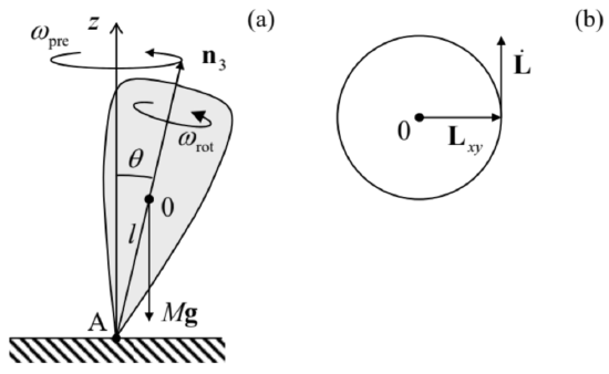
Figure 4.9. Symmetric top in the gravity field: (a) a side view at the system and (b) the top view at the evolution of the horizontal component of the angular momentum vector.

The uniform gravity field \(\mathbf{g}\) creates bulk-distributed forces that, as we know from the analysis of the physical pendulum in Sec. 3, are equivalent to a single force \(M \mathbf{g}\) applied in the center of mass - in Figure 9 , point 0 . The torque of this force relative to the support point \(\mathrm{A}\) is \[\boldsymbol{\tau}=\left.\mathbf{r}_{0}\right|_{\text {in } \mathrm{A}} \times M \mathbf{g}=M l \mathbf{n}_{3} \times \mathbf{g} .\]

Hence the general equation (33) of the angular momentum evolution (valid in any inertial frame, for example the one with an origin in point A) becomes \[\dot{\mathbf{L}}=M l \mathbf{n}_{3} \times \mathbf{g} .\] Despite the apparent simplicity of this (exact!) equation, its analysis is straightforward only in the limit when the top is launched spinning about its symmetry axis \(\mathbf{n}_{3}\) with a very high angular velocity \(\omega_{\text {rot. }}\). In this case, we may neglect the contribution to \(\mathbf{L}\) due to a relatively small precession velocity \(\omega_{\text {pre }}\) (still to be calculated), and use Eq. (26) to write \[\mathbf{L}=I_{3} \boldsymbol{\omega}=I_{3} \omega_{\mathrm{rot}} \mathbf{n}_{3} .\] Then Eq. (70) shows that the vector \(\mathbf{L}\) is perpendicular to both \(\mathbf{n}_{3}\) (and hence \(\mathbf{L}\) ) and \(\mathbf{g}\), i.e. lies within the horizontal plane and is perpendicular to the horizontal component \(\mathbf{L}_{x y}\) of the vector \(\mathbf{L}-\) see Figure \(9 \mathrm{~b}\). Since, according to Eq. (70), the magnitude of this vector is constant, \(|\mathbf{L}|=m g l \sin \theta\), the vector \(\mathbf{L}\) (and hence the body’s main axis) rotates about the vertical axis with the following angular velocity:

\(\begin{aligned}&\text { Torque- } \\&\text { induced } \\&\text { ecession: } \\&\text { fintion } \\&\text { limit }\end{aligned} \quad \omega_{\text {pre }}=\frac{|\dot{\mathbf{L}}|}{L_{x y}}=\frac{M g l \sin \theta}{L \sin \theta} \equiv \frac{M g l}{L}=\frac{M g l}{I_{3} \omega_{\text {rot }}} .\)

Thus, very counter-intuitively, the fast-rotating top does not follow the external, vertical force and, in addition to fast spinning about the symmetry axis \(\mathbf{n}_{3}\), performs a revolution, called the torqueinduced precession, about the vertical axis. Note that, similarly to the free-precession frequency (59), the torque-induced precession frequency \((72)\) does not depend on the initial (and sustained) angle \(\theta\). However, the torque-induced precession frequency is inversely (rather than directly) proportional to \(\omega_{\text {rot }}\). This fact makes the above simple theory valid in many practical cases. Indeed, Eq. (71) is quantitatively valid if the contribution of the precession into \(\mathbf{L}\) is relatively small: \(I \omega_{\text {pre }} \ll I_{3} \omega_{\text {rot }}\), where \(I\) is a certain effective moment of inertia for the precession - to be calculated below. Using Eq. (72), this condition may be rewritten as \[\omega_{\mathrm{rot}}>>\left(\frac{M g l I}{I_{3}^{2}}\right)^{1 / 2} .\] According to Eq. (16), for a body of not too extreme proportions, i.e. with all linear dimensions of the order of the same length scale \(l\), all inertia moments are of the order of \(M l^{2}\), so that the right-hand side of Eq. \((73)\) is of the order of \((g / l)^{1 / 2}\), i.e. comparable with the frequency of small oscillations of the same body as the physical pendulum, i.e. at the absence of its fast rotation.

To develop a qualitative theory that would be valid beyond such approximate treatment, the Euler equations (66) may be used, but are not very convenient. A better approach, suggested by the same L. Euler, is to introduce a set of three independent angles between the principal axes \(\left\{\mathbf{n}_{1}, \mathbf{n}_{2}, \mathbf{n}_{3}\right\}\) bound to the rigid body, and the axes \(\left\{\mathbf{n}_{x}, \mathbf{n}_{y}, \mathbf{n}_{z}\right\}\) of an inertial reference frame (Figure 10), and then express the basic equation (33) of rotation, via these angles. There are several possible options for the definition of such angles; Figure 10 shows the set of Euler angles, most convenient for analyses of fast rotation. \({ }^{18}\) As one can see, the first Euler angle, \(\theta\), is the usual polar angle measured from the \(\mathbf{n}_{z}\)-axis to the \(\mathbf{n}_{3}\)-axis. The second one is the azimuthal angle \(\varphi\), measured from the \(\mathbf{n}_{x}\)-axis to the so-called line of nodes formed by the intersection of planes \(\left[\mathbf{n}_{x}, \mathbf{n}_{y}\right]\) and \(\left[\mathbf{n}_{1}, \mathbf{n}_{2}\right]\). The last Euler angle, \(\psi\), is measured Euler within the plane \(\left[\mathbf{n}_{1}, \mathbf{n}_{2}\right]\), from the line of nodes to axis \(\mathbf{n}_{1}\)-axis. For example, in the simple picture of slow force-induced precession of a symmetric top, that was discussed above, the angle \(\theta\) is constant, the angle \(\psi\) changes rapidly, with the rotation velocity \(\omega_{\mathrm{rot}}\), while the angle \(\varphi\) evolves with the precession frequency \(\omega_{\text {pre }}(72)\).

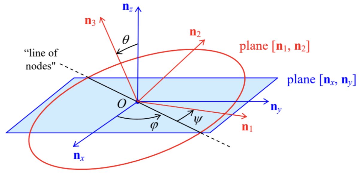Fig. 4.10. Definition of the Euler angles.

Now we can express the principal-axes components of the instantaneous angular velocity vector, \(\omega_{1}, \omega_{2}\), and \(\omega_{3}\), as measured in the lab reference frame, in terms of the Euler angles. This may be readily done by calculating, from Figure 10, the contributions of the Euler angles’ evolution to the rotation about each principal axis, and then adding them up: \[\begin{aligned} &\omega_{1}=\dot{\varphi} \sin \theta \sin \psi+\dot{\theta} \cos \psi \\ &\omega_{2}=\dot{\varphi} \sin \theta \cos \psi-\dot{\theta} \sin \psi \\ &\omega_{3}=\dot{\varphi} \cos \theta+\dot{\psi} \end{aligned}\] These relations enable the expression of the kinetic energy of rotation \((25)\) and the angular momentum components (26) via the generalized coordinates \(\theta, \varphi\), and \(\psi\) and their time derivatives (i.e. the corresponding generalized velocities), and then using the powerful Lagrangian formalism to derive their equations of motion. This is especially simple to do in the case of symmetric tops (with \(I_{1}=I_{2}\) ), because plugging Eqs. (74) into Eq. (25) we get an expression, \[T_{\text {rot }}=\frac{I_{1}}{2}\left(\dot{\theta}^{2}+\dot{\varphi}^{2} \sin ^{2} \theta\right)+\frac{I_{3}}{2}(\dot{\varphi} \cos \theta+\dot{\psi})^{2},\] which does not include explicitly either \(\varphi\) or \(\psi\). (This reflects the fact that for a symmetric top we can always select the \(\mathbf{n}_{1}\)-axis to coincide with the line of nodes, and hence take \(\psi=0\) at the considered moment of time. Note that this trick does not mean we can take \(\dot{\psi}=0\), because the \(\mathbf{n}_{1}\)-axis, as observed from an inertial reference frame, moves!) Now we should not forget that at the torque-induced precession, the center of mass moves as well (see, e.g., Figure 9), so that according to Eq. (14), the total kinetic energy of the body is the sum of two terms, \[T=T_{\text {rot }}+T_{\text {tran }}, \quad T_{\text {tran }}=\frac{M}{2} V^{2}=\frac{M}{2} l^{2}\left(\dot{\theta}^{2}+\dot{\varphi}^{2} \sin ^{2} \theta\right),\] while its potential energy is just \[U=M g l \cos \theta+\text { const } \text {. }\] Now we could readily write the Lagrange equations of motion for the Euler angles, but it is simpler to immediately notice that according to Eqs. (75)-(77), the Lagrangian function, \(T-U\), does not depend explicitly on the "cyclic" coordinates \(\varphi\) and \(\psi\), so that the corresponding generalized momenta (2.31) are conserved: \[\begin{gathered} p_{\varphi} \equiv \frac{\partial T}{\partial \dot{\varphi}}=I_{\mathrm{A}} \dot{\varphi} \sin ^{2} \theta+I_{3}(\dot{\varphi} \cos \theta+\dot{\psi}) \cos \theta=\mathrm{const}, \\ p_{\psi} \equiv \frac{\partial T}{\partial \dot{\psi}}=I_{3}(\dot{\varphi} \cos \theta+\dot{\psi})=\mathrm{const}, \end{gathered}\] where \(I_{\mathrm{A}} \equiv I_{1}+M l^{2}\). (According to Eq. (29), \(I_{\mathrm{A}}\) is just the body’s moment of inertia for rotation about a horizontal axis passing through the support point A.) According to the last of Eqs. (74), \(p_{\psi}\) is just \(L_{3}\), i.e. the angular momentum’s component along the precessing axis \(\mathbf{n}_{3}\). On the other hand, by its very definition (78), \(p_{\varphi}\) is \(L_{z}\), i.e. the same vector \(\mathbf{L}\) ’s component along the static axis \(z\). (Actually, we could foresee in advance the conservation of both these components of \(\mathbf{L}\) for our system, because the vector (69) of the external torque is perpendicular to both \(\mathbf{n}_{3}\) and \(\mathbf{n}_{z}\).) Using this notation, and solving the simple system of linear equations (78)-(79) for the angle derivatives, we get \[\dot{\varphi}=\frac{L_{z}-L_{3} \cos \theta}{I_{\mathrm{A}} \sin ^{2} \theta}, \quad \dot{\psi}=\frac{L_{3}}{I_{3}}-\frac{L_{z}-L_{3} \cos \theta}{I_{\mathrm{A}} \sin ^{2} \theta} \cos \theta .\] One more conserved quantity in this problem is the full mechanical energy \({ }^{19}\) \[E \equiv T+U=\frac{I_{\mathrm{A}}}{2}\left(\dot{\theta}^{2}+\dot{\varphi}^{2} \sin ^{2} \theta\right)+\frac{I_{3}}{2}(\dot{\varphi} \cos \theta+\dot{\psi})^{2}+M g l \cos \theta \text {. }\] Plugging Eqs. (80) into Eq. (81), we get a first-order differential equation for the angle \(\theta\), which may be represented in the following physically transparent form: \[\frac{I_{\mathrm{A}}}{2} \dot{\theta}^{2}+U_{\mathrm{ef}}(\theta)=E, \quad U_{\mathrm{ef}}(\theta) \equiv \frac{\left(L_{z}-L_{3} \cos \theta\right)^{2}}{2 I_{\mathrm{A}} \sin ^{2} \theta}+\frac{L_{3}^{2}}{2 I_{3}}+M g l \cos \theta+\text { const }\] Thus, similarly to the planetary problems considered in Sec. 3.4, the torque-induced precession of a symmetric top has been reduced (without any approximations!) to a 1D problem of the motion of one of its degrees of freedom, the polar angle \(\theta\), in the effective potential \(U_{\mathrm{ef}}(\theta)\). According to Eq. (82), very similar to Eq. (3.44) for the planetary problem, this potential is the sum of the actual potential energy \(U\) given by Eq. (77), and a contribution from the kinetic energy of motion along two other angles. In the absence of rotation about the axes \(\mathbf{n}_{z}\) and \(\mathbf{n}_{3}\) (i.e., \(L_{z}=L_{3}=0\) ), Eq. (82) is reduced to the first integral of the equation (40) of motion of a physical pendulum, with \(I^{\prime}=I_{\mathrm{A}}\). If the rotation is present, then (besides the case of very special initial conditions when \(\theta(0)=0\) and \(\left.L_{z}=L_{3}\right),{ }^{20}\) the first contribution to \(U_{\mathrm{ef}}(\theta)\) diverges at \(\theta \rightarrow 0\) and \(\pi\), so that the effective potential energy has a minimum at some non-zero value \(\theta_{0}\) of the polar angle \(\theta\) - see Figure 11 .

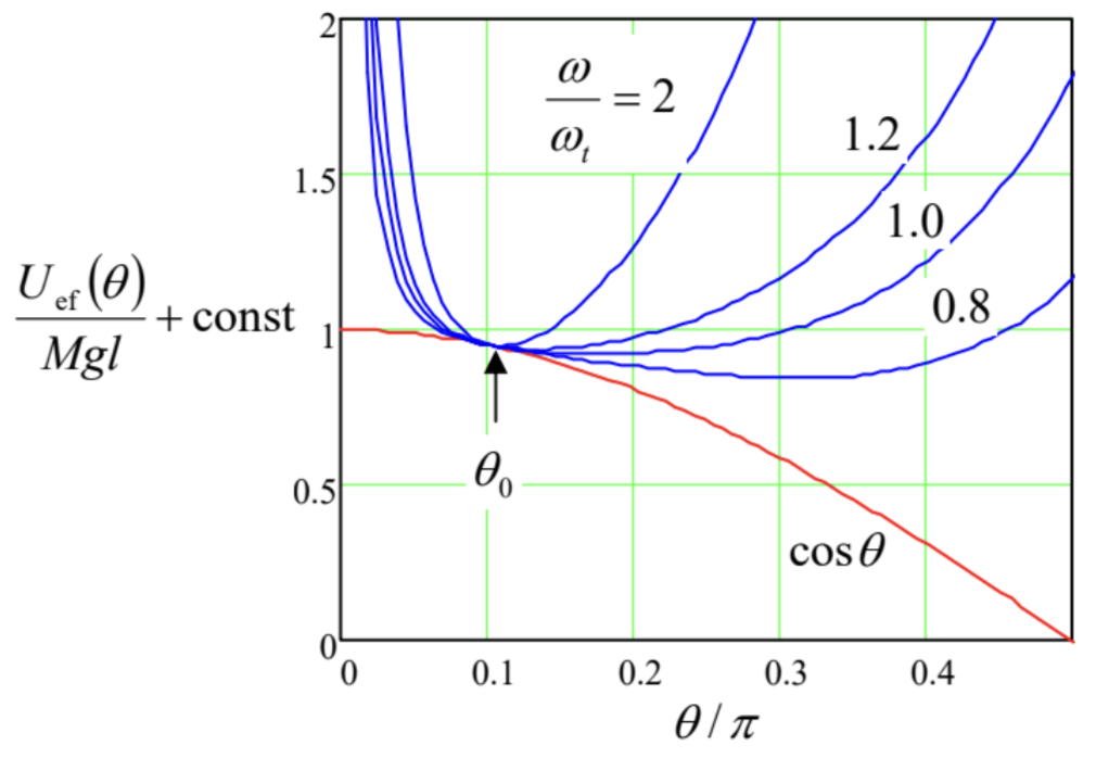
Figure 4.11. The effective potential energy \(U_{\text {ef }}\) of the symmetric top, given by Eq. (82), as a function of the polar angle \(\theta\), for a particular value (0.95) of the ratio \(r \equiv L_{z} / L_{3}\) (so that at \(\omega_{\text {rot }}>>\) \(\left.\omega_{\mathrm{h}}, \theta_{0}=\cos ^{-1} r \approx 0.1011 \pi\right)\), and several values of the ratio \(\omega_{\mathrm{rot}} / \omega_{\mathrm{th}}\).

If the initial angle \(\theta(0)\) is equal to this value \(\theta_{0}\), i.e. if the initial effective energy is equal to its minimum value \(U_{\mathrm{ef}}\left(\theta_{0}\right)\), the polar angle remains constant through the motion: \(\theta(t)=\theta_{0}\). This corresponds to the pure torque-induced precession whose angular velocity is given by the first of Eqs. (80): \[\omega_{\mathrm{pre}} \equiv \dot{\varphi}=\frac{L_{z}-L_{3} \cos \theta_{0}}{I_{\mathrm{A}} \sin ^{2} \theta_{0}} .\] The condition for finding \(\theta_{0}, d U_{\mathrm{ef}} / d \theta=0\), is a transcendental algebraic equation that cannot be solved analytically for arbitrary parameters. However, in the high spinning speed limit (73), this is possible. Indeed, in this limit the \(M g l\)-proportional contribution to \(U_{\text {ef }}\) is small, and we may analyze its effect by successive approximations. In the \(0^{\text {th }}\) approximation, i.e. at \(M g l=0\), the minimum of \(U_{\text {ef }}\) is evidently achieved at \(\cos \theta_{0}=L_{z} / L_{3}\), turning the precession frequency (83) to zero. In the next, \(1^{\text {st }}\) approximation, we may require that at \(\theta=\theta_{0}\), the derivative of the first term of Eq. (82) for \(U_{\text {ef }}\) over \(\cos \theta\), equal to \(L_{z}\left(L_{z}-L_{3} \cos \theta\right) / I_{\mathrm{A}} \sin ^{2} \theta_{,}^{21}\) is canceled with that of the gravity-induced term, equal to \(M g l\). This immediately yields \(\omega_{\text {pre }}=\left(L_{z}-L_{3} \cos \theta_{0}\right) / I_{\mathrm{A}} \sin ^{2} \theta_{0}=M g l / L_{3}\), so that identifying \(\omega_{\text {rot }}\) with \(\omega_{3} \equiv L_{3} / I_{3}\) (see Figure 8), we recover the simple expression (72).

The second important result that may be readily obtained from Eq. (82) is the exact expression for the threshold value of the spinning speed for a vertically rotating top \(\left(\theta=0, L_{z}=L_{3}\right)\). Indeed, in the limit \(\theta \rightarrow 0\) this expression may be readily simplified: \[U_{\text {ef }}(\theta) \approx \text { const }+\left(\frac{L_{3}^{2}}{8 I_{\mathrm{A}}}-\frac{M g l}{2}\right) \theta^{2} .\] This formula shows that if \(\omega_{\mathrm{rot}} \equiv L_{3} / I_{3}\) is higher than the following threshold value,

\[\ \text{Threshold rotation speed}\quad\quad\quad\quad\omega_{\mathrm{th}} \equiv 2\left(\frac{M g l I_{\mathrm{A}}}{I_{3}^{2}}\right)^{1 / 2},\]

then the coefficient at \(\theta^{2}\) in Eq. (84) is positive, so that \(U_{\text {ef }}\) has a stable minimum at \(\theta_{0}=0\). On the other hand, if \(\omega_{3}\) is decreased below \(\omega_{\mathrm{th}}\), the fixed point becomes unstable, so that the top falls. As the plots in Figure 11 show, Eq. (85) for the threshold frequency works very well even for non-zero but small values of the precession angle \(\theta_{0}\). Note that if we take \(I=I_{\mathrm{A}}\) in the condition \((73)\) of the approximate treatment, it acquires a very simple sense: \(\omega_{\mathrm{rot}}>>\omega_{\mathrm{th}}\).

Finally, Eqs. (82) give a natural description of one more phenomenon. If the initial energy is larger than \(U_{\mathrm{ef}}\left(\theta_{0}\right)\), the angle \(\theta\) oscillates between two classical turning points on both sides of the fixed point \(\theta_{0}\)-see also Figure 11. The law and frequency of these oscillations may be found exactly as in Sec. \(3.3\) - see Eqs. (3.27) and (3.28). At \(\omega_{3} \gg \omega_{\mathrm{h}}\), this motion is a fast rotation of the symmetry axis \(\mathbf{n}_{3}\) of the body about its average position performing the slow torque-induced precession. Historically, these oscillations are called nutations, but their physics is similar to that of the free precession that was analyzed in the previous section, and the order of magnitude of their frequency is given by Eq. (59).

It may be proved that small friction (not taken into account in the above analysis) leads first to decay of these nutations, then to a slower drift of the precession angle \(\theta_{0}\) to zero and, finally, to a gradual decay of the spinning speed \(\omega_{\mathrm{rot}}\) until it reaches the threshold (85) and the top falls.

---

\({ }^{19}\) Of the several choices more convenient in the absence of fast rotation, the most common is the set of so-called Tait-Brian angles (called the yaw, pitch, and roll), which are broadly used for aircraft and maritime navigation.

\({ }^{20}\) Indeed, since the Lagrangian does not depend on time explicitly, \(H=\) const, and since the full kinetic energy \(T\) (75)-(76) is a quadratic-homogeneous function of the generalized velocities, \(E=H\).

\({ }^{21}\) In that simple case, the body continues to rotate about the vertical symmetry axis: \(\theta(t)=0\). Note, however, that such motion is stable only if the spinning speed is sufficiently high - see Eq. (85) below.

\({ }^{22}\) Indeed, the derivative of the fraction \(1 / 2 I_{\mathrm{A}} \sin ^{2} \theta\), taken at the point \(\cos \theta=L_{z} / L_{3}\), is multiplied by the numerator, \(\left(L_{z}-L_{3} \cos \theta\right)^{2}\), which turns to zero at this point.