6.8: Exercise Problems

For each of the systems specified in Problems 6.1-6.6:

(i) introduce convenient generalized coordinates \(q_{j}\) of the system,

(ii) calculate the frequencies of its small harmonic oscillations near the equilibrium,

(iii) calculate the corresponding distribution coefficients, and

(iv) sketch the oscillation modes.

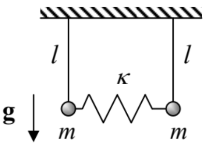
6.1. Two elastically coupled pendula, confined to a vertical plane, with the parameters shown in the figure on the right (see also Problems \(1.8\) and 2.9).

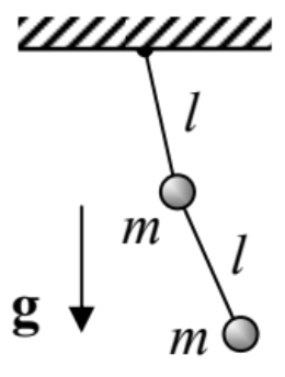
6.2. The double pendulum, confined to a vertical plane containing the support point (considered in Problem 2.1), with \(m^{\prime}=m\) and \(l=l^{\prime}-\) see the figure on the right.

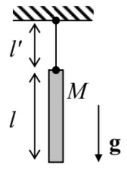
6.3. The chime bell considered in Problem \(4.8\) (see the figure on the right), for the particular case \(l=l^{\prime}\).

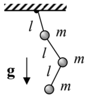
6.4. The triple pendulum shown in the figure on the right, with the motion confine to a vertical plane containing the support point.

Hint: You may use any (e.g., numerical) method to calculate the characteristic equation’s roots.

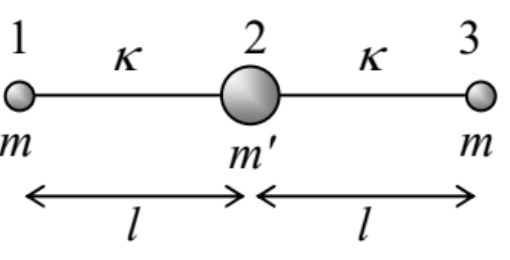
6.5. A linear, symmetric system of three particles, shown in the figure on the right, where the connections between the particles not only act as usual elastic springs (giving potential energies \(U=\kappa(\Delta l)^{2} / 2\) ) but also resist bending, giving additional potential energy \(U^{\prime}=\kappa^{\prime}(l \theta)^{2} / 2\), where \(\theta\) is the (small) bending angle. \({ }^{33}\)

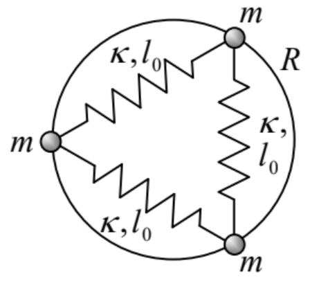
6.6. Three similar beads of mass \(m\), which may slide along a circle of radius \(R\) without friction, connected with similar springs with elastic constants \(\kappa\) and equilibrium lengths \(l_{0}\) - see the figure on the right.

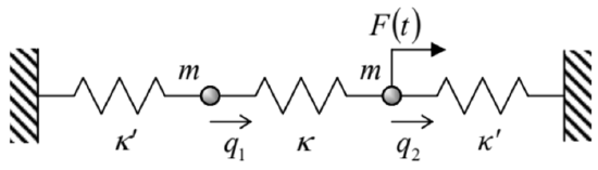
6.7. An external longitudinal force \(F(t)\) is applied to the right particle of the system shown in Figure 1, with \(\kappa_{\mathrm{L}}=\kappa_{\mathrm{R}}=\kappa^{\prime}\) and \(m_{1}=m_{2} \equiv m\) (see the figure on the right), and the response \(q_{1}(t)\) of the left \(N\) particle to this force is being measured.

(i) Calculate the temporal Green’s function for this response.

(ii) Use this function to calculate the response to the following force: \[F(t)= \begin{cases}0, & \text { for } t<0 \\ F_{0} \sin \omega t, & \text { for } 0 \leq t\end{cases}\] with constant amplitude \(F_{0}\) and frequency \(\omega\).

\(\underline{6.8}\). Use the Lagrangian formalism to re-derive Eqs. (24) for both the longitudinal and the transverse oscillations in the system shown in Figure \(4 \mathrm{a}\).

6.9. Calculate the energy (per unit length) of a sinusoidal traveling wave propagating in the 1D system shown in Figure 4a. Use your result to calculate the average power flow created by the wave, and compare it with Eq. (49) valid in the acoustic wave limit.

6.10. Calculate the spatial distributions of the kinetic and potential energies in a standing, sinusoidal, 1D acoustic wave, and analyze their evolution in time.

6.11. The midpoint of a guitar string of length \(l\) has been slowly pulled off by distance \(h<<l\) from its equilibrium position, and then let go. Neglecting dissipation, use two different approaches to calculate the midpoint’s displacement as a function of time.

Hint: You may like to use the following table series: \[\sum_{m=1}^{\infty} \frac{\cos (2 m-1) \xi}{(2 m-1)^{2}}=\frac{\pi^{2}}{8}\left(1-\frac{\xi}{\pi / 2}\right), \quad \text { for } 0 \leq \xi \leq \pi .\]

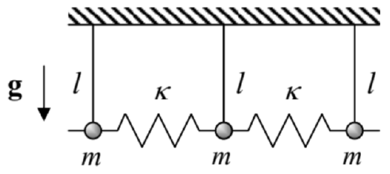
6.12. Calculate the dispersion law \(\omega(k)\) and the maximum and minimum frequencies of small longitudinal waves in a long chain of similar, spring-coupled pendula - see the figure on the right.

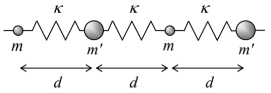
6.13. Calculate and analyze the dispersion relation \(\omega(k)\) for small waves in a long chain of elastically coupled particles with alternating masses - see the figure on the right. In particular, discuss the dispersion relation’s period \(\Delta k\), and its evolution at \(m^{\prime} \rightarrow m\).

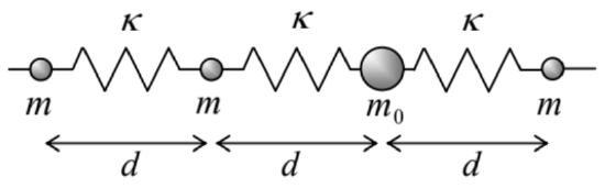
6.14. Analyze the traveling wave’s reflection from a "point inhomogeneity": a single particle with a different mass \(m_{0} \neq m\), within an otherwise uniform 1D chain - see the figure on the right.

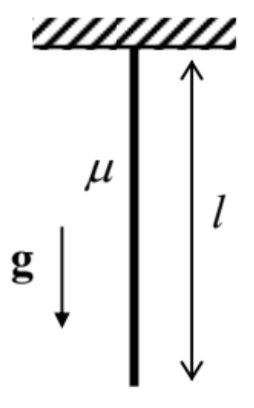
6.15*

(i) Explore an approximate way to analyze waves in a continuous \(1 \mathrm{D}\) system with parameters slowly varying along its length.

(ii) Apply this method to calculate the frequencies of transverse standing waves on a freely hanging heavy rope of length \(l\), with a constant mass \(\mu\) per unit length - see the figure on the right.

(iii) For the three lowest standing wave modes, compare the results with those obtained in the solution of Problem 4 for the triple pendulum.

Hint: The reader familiar with the WKB approximation in quantum mechanics (see, e.g., QM Sec. 2.4) is welcome to adapt it for this classical application. Another possible starting point is the van der Pol approximation discussed in Sec. 5.3, which should be translated from the time domain to the space domain.

6.16. \({ }^{*}\) Use the van der Pol approximation to analyze the mutual phase locking of two weakly coupled self-oscillators with the dissipative nonlinearity, for the cases of:

(i) the direct coordinate coupling, described by Eq. (5), and

(ii) a bilinear but otherwise arbitrary coupling of two similar oscillators.

Hint: In Task (ii), describe the coupling by a linear operator, and express the result via its Fourier image.

6.17. \({ }^{*}\) Extend the second task of the previous problem to the mutual phase locking of \(N\) similar self-oscillators. In particular, explore the in-phase mode’s stability for the case of the so-called global coupling via a single force \(F\) contributed equally by all oscillators.

6.18. \({ }^{*}\) Find the condition of non-degenerate parametric excitation in a system of two coupled oscillators, described by Eqs. (5), but with a time-dependent coupling: \(\kappa \rightarrow \kappa\left(1+\mu \cos \omega_{\mathrm{p}} t\right)\), with \(\omega_{\mathrm{p}} \approx\) \(\Omega_{1}+\Omega_{2}\), and \(\kappa / m<<\left|\Omega_{2}-\Omega_{1}\right|\).

Hint: Assuming the modulation depth \(\mu\), static coupling \(\kappa\), and detuning \(\xi \equiv \omega_{\mathrm{p}}-\left(\Omega_{1}+\Omega_{2}\right)\) sufficiently small, use the van der Pol approximation for each of the coupled oscillators.

6.19. Show that the cubic nonlinearity of the type \(\alpha q^{3}\) indeed enables the parametric interaction ("four-wave mixing") of oscillations with incommensurate frequencies related by Eqs. (92a).

6.20. Calculate the velocity of the transverse waves propagating on a thin, planar, elastic membrane, with mass \(m\) per unit area, pre-stretched with force \(\tau\) per unit width.

---

\({ }^{33}\) This is a good model for small oscillations of linear molecules such as the now-infamous \(\mathrm{CO}_{2}\).