
11.12: Two-body Scattering


- Last updated
- Mar 14, 2021
- Save as PDF

( \newcommand{\kernel}{\mathrm{null}\,}\)
Two moving bodies, that are interacting via a central force, scatter when the force is repulsive, or when an attractive system is unbound. Two-body scattering of bodies is encountered extensively in the fields of astronomy, atomic, nuclear, and particle physics. The probability of such scattering is most conveniently expressed in terms of scattering cross sections defined below.
Total two-body scattering cross section
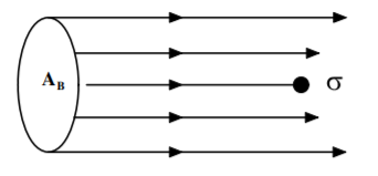
The concept of scattering cross section for two-body scattering is most easily described for the total two-body cross section. The probability P that a beam of nB incident point particles/second, distributed over a cross sectional area AB, will hit a single solid object, having a cross sectional area σ, is given by the ratio of the areas as illustrated in Figure 11.12.1. That is,
P=σAB
where it is assumed that AB>>σ. For a spherical target body of radius r, the cross section σ=πr2. The scattering probability P is proportional to the cross section σ which is the cross section of the target body perpendicular to the beam; thus σ has the units of area.
Since the incident beam of nB incident point particles/second, has a cross sectional area AB, then it will have an areal density I given by
I=nBAB beam particles/m2/s
The number of beam particles scattered per second NS by this single target scatterer equals
NS=PnB=σABIAB=σI
Thus the cross section for scattering by this single target body is
σ=NSI=Scattered particles/sincident beam/m2/s
Realistically one will have many target scatterers in the target and the total scattering probability increases proportionally to the number of target scatterers. That is, for a target comprising an areal density of ηT target bodies per unit area of the incident beam, then the number scattered will increase proportional to the target areal density ηT. That is, there will be ηTAB scattering bodies that interact with the beam assuming that the target has a larger area than the beam. Thus the total number scattered per second NS by a target that comprises multiple scatterers is
NS=σnBABηTAB=σnBηT
Note that this is independent of the cross sectional area of the beam assuming that the target area is larger than that of the beam. That is, the number scattered per second is proportional to the cross section σ times the product of the number of incident particles per second, nB, and the areal density of target scatterers, ηT. Typical cross sections encountered in astrophysics are σ≈1014m2, in atomic physics: σ≈10−20m2, and in nuclear physics; σ≈10−28m2=barns.3
N. B., the above proof assumed that the target size is larger than the cross sectional area of the incident beam. If the size of the target is smaller than the beam, then nB is replaced by the areal density/s of the beam ηB and ηT is replaced by the number of target particles nT and the cross-sectional size of the target cancels.
Differential two-body scattering cross section
The differential two-body scattering cross section gives much more detailed information of the scattering force than does the total cross section because of the correlation between the impact parameter and the scattering angle. That is, a measurement of the number of beam particles scattered into a given solid angle as a function of scattering angles θ,ϕ probes the radial form of the scattering force.
The differential cross section for scattering of an incident beam by a single target body into a solid angle dΩ at scattering angles θ,ϕ is defined to be
dσdΩ(θϕ)≡1IdNS(θ,ϕ)dΩ
where the right-hand side is the ratio of the number scattered per target nucleus into solid angle dΩ(θ,ϕ), to the incident beam intensity I particles/m2/s.
Similar reasoning used to derive Equation ??? leads to the number of beam particles scattered into a solid angle dΩ for nB beam particles incident upon a target with areal density ηT is dNS(θ,ϕ)dΩ=nBηTdσdΩ(θϕ)
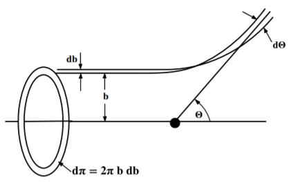
Consider the equivalent one-body system for scattering of one body by a scattering force center in the center of mass. As shown in figures (11.8.2) and 11.12.2, the perpendicular distance between the center of force of the two body system and trajectory of the incoming body at infinite distance is called the impact parameter b. For a central force the scattering system has cylindrical symmetry, therefore the solid angle dΩ(θϕ)=sinθdθdϕ can be integrated over the azimuthal angle ϕ to give dΩ(θ)=2πsinθdθ.
For the inverse-square, two-body, central force there is a one-to-one correspondence between impact parameter b and scattering angle θ for a given bombarding energy. In this case, assuming conservation of flux means that the incident beam particles passing through the impact-parameter annulus between b and b+db must equal the the number passing between the corresponding angles θ and θ+dθ. That is, for an incident beam flux of I particles/m2/s the number of particles per second passing through the annulus is
I2πb|db|=2πdσdΩIsinθ|dθ|
The modulus is used to ensure that the number of particles is always positive. Thus dσdΩ=bsinθ|dbdθ|
Impact parameter dependence on scattering angle
If the function b=f(θ,Ecm) is known, then it is possible to evaluate |dbdθ| which can be used in Equation ??? to calculate the differential cross section. A simple and important case to consider is two-body elastic scattering for the inverse-square law force such as the Coulomb or gravitational forces. To avoid confusion in the following discussion, the center-of-mass scattering angle will be called θ, while the angle used to define the hyperbolic orbits in the discussion of trajectories for the inverse square law, will be called ψ.
In chapter 11.8 the equivalent one-body representation gave that the radial distance for a trajectory for the inverse square law is given by
1r=−μkl2[1+ϵcosψ]
Note that closest approach occurs when ψ=0 while for r→∞ the bracket must equal zero, that is
cosψ∞=±|1ϵ|
The polar angle ψ is measured with respect to the symmetry axis of the two-body system which is along the line of distance of closest approach as shown in Figure (11.8.2). The geometry and symmetry show that the scattering angle θ is related to the trajectory angle ψ∞ by
θ=π−2ψ∞
Equation (11.7.1) gives that
ψ∞=∫∞rmin±ldrr2√2μ(Ecm−U−l22μr2)
Since
l2=b2p2=b22μEcm
then the scattering angle can be written as.
ψ∞=π−θ2=∫∞rminbdrr2√(1−UEcm−b2r2)
Let u=1r, then ψ∞=π−θ2=∫∞rminbdu√(1−UEcm−b2u2)
For the repulsive inverse square law
U=−kr=−ku
where k is taken to be positive for a repulsive force. Thus the scattering angle relation becomes ψ∞=π−θ2=∫∞rminbdu√(1+kuEcm−b2u2)
The solution of this equation is given by equation (11.8.12) to be
u=1r=−μkl2[1+ϵcosψ]
where the eccentricity
ϵ=√1+2Ecml2μk2
For r→∞, u=0 then, as shown previously,
|1ϵ|=cosψ∞=cosπ−θ2=sinθ2
Therefore
2Ecmbk=√ϵ2−1=cotθ2
that is, the impact parameter b is given by the relation
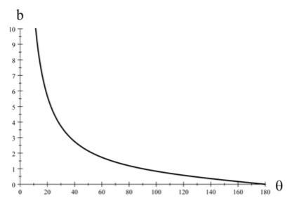
b=k2Ecmcotθ2
Thus, for an inverse-square law force, the two-body scattering has a one-to-one correspondence between impact parameter b and scattering angle θ as shown schematically in Figure 11.12.3.
If k is negative, which corresponds to an attractive inverse square law, then one gets the same relation between impact parameter and scattering angle except that the sign of the impact parameter b is opposite. This means that the hyperbolic trajectory has an interior rather than exterior focus. That is, the trajectory partially orbits around the center of force rather than being repelled away.
rmin=k2Ecm(1+1sinθ2)
Note that for θ=180o then
Ecm=krmin=U(rmin)
which is what you would expect from equating the incident kinetic energy to the potential energy at the distance of closest approach.
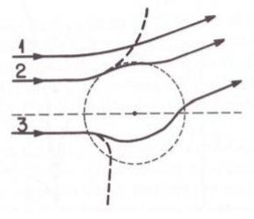
For scattering of two nuclei by the repulsive Coulomb force, if the impact parameter becomes small enough, the attractive nuclear force also acts leading to impact-parameter dependent effective potentials illustrated in Figure 11.12.4. Trajectory 1 does not overlap the nuclear force and thus is pure Coulomb. Trajectory 2 interacts at the periphery of the nuclear potential and the trajectory deviates from pure Coulomb shown dashed. Trajectory 3 passes through the interior of the nuclear potential. These three trajectories all can lead to the same scattering angle and thus there no longer is a one-to-one correspondence between scattering angle and impact parameter.
Rutherford scattering
Two models of the nucleus evolved in the 1900’s, the Rutherford model assumed electrons orbiting around a small nucleus like planets around the sun, while J.J. Thomson’s ”plum-pudding” model assumed the electrons were embedded in a uniform sphere of positive charge the size of the atom. When Rutherford derived his classical formula in 1911 he realized that it can be used to determine the size of the nucleus since the electric field obeys the inverse square law only when outside of the charged spherical nucleus. Inside a uniform sphere of charge the electric field is E∝r and thus the scattering cross section will not obey the Rutherford relation for distances of closest approach that are less than the radius of the sphere of negative charge. Observation of the angle beyond which the Rutherford formula breaks down immediately determines the radius of the nucleus.
dσdΩ=14(k2Ecm)21sin4θ2
This cross section assumes elastic scattering by a repulsive two-body inverse-square central force. For scattering of nuclei in the Coulomb potential, the constant k is given to be k=ZpZTe24πεo
The cross section, scattering angle and Ecm of Equation ??? are evaluated in the center-of-mass coordinate system, whereas usually two-body elastic scattering data involve scattering of the projectiles by a stationary target as discussed in chapter 11.13.
Gieger and Marsden performed scattering of 7.7 MeV α particles from a thin gold foil and proved that the differential scattering cross section obeyed the Rutherford formula back to angles corresponding to a distance of closest approach of 10−14m which is much smaller that the 10−10m size of the atom. This validated the Rutherford model of the atom and immediately led to the Bohr model of the atom which played such a crucial role in the development of quantum mechanics. Bohr showed that the agreement with the Rutherford formula implies the Coulomb field obeys the inverse square law to small distances. This work was performed at Manchester University, England between 1908 and 1913. It is fortunate that the classical result is identical to the quantal cross section for scattering, otherwise the development of modern physics could have been delayed for many years.
Scattering of very heavy ions, such as 208Pb, can electromagnetically excite target nuclei. For the Coulomb force the impact parameter b and the distance of closest approach, rmin are directly related to the scattering angle θ by Equation ???. Thus observing the angle of the scattered projectile unambiguously determines the hyperbolic trajectory and thus the electromagnetic impulse given to the colliding nuclei. This process, called Coulomb excitation, uses the measured angular distribution of the scattered ions for inelastic excitation of the nuclei to precisely and unambiguously determine the Coulomb excitation cross section as a function of impact parameter. This unambiguously determines the shape of the nuclear charge distribution.
Example 11.12.1: Two-body scattering by an inverse cubic force
Assume two-body scattering by a potential U=kr2 where k>0. This corresponds to a repulsive two-body force F=2kr3ˆr. Insert this force into Binet’s differential orbit, equation (11.5.5), gives
d2udϕ2+u(1+2kμl2)=0
The solution is of the form u=Asin(ωψ+β) where A and β are constants of integration, l=μr2˙ψ, and
ω2=(1+2kμl2)
Initially r=∞, u=0, and therefore β=0. Also at r=∞, E=12μ˙r2∞, that is |˙r∞|=√2Eμ. Then
˙r=drdψ˙ψ=drdψlμr2=−lμdudψ=−Alμωcos(ωψ)
The initial energy gives that A=1lω√2μE. Hence the orbit equation is
u=1r=√2μElωsin(ωψ)
The above trajectory has a distance of closest approach, rmin, when ψmin=π2ω. Moreover, due to the symmetry of the orbit, the scattering angle θ is given by
θ=π−2ψ0=π(1−1ω)
Since l2=μ2b2˙r2∞=2b2μE then
1−θπ=(1+2kμl2)−12=(1+kb2E)−12
This gives that the impact parameter b is related to scattering angle by
b2=kE(π−θ)2(2π−θ)θ
This impact parameter relation can be used in Equation ??? to give the differential cross section
dσdΩ=bsinθ|dbdθ|=kEsinθπ2(π−θ)(2π−θ)2θ2
These orbits are called Cotes spirals.
3The term "barn" was chosen because nuclear physicists joked that the cross sections for neutron scattering by nuclei were as large as a barn door.