
11.4: Transmission Lines in General


- Last updated
- Jun 21, 2021
- Save as PDF

( \newcommand{\kernel}{\mathrm{null}\,}\)
Relations similar to Equations (11.3.8,11.3.9, and 11.3.10) are valid for a transmission line constructed of arbitrarily shaped conductors. In the general case it is convenient to describe the properties of a lossless line in terms of the inductance per unit length, L Henries/m, and the capacitance per unit length,
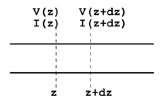
C Farads/m. One can write the appropriate transmission line equations using ordinary circuit theory. If the current on the line changes with time there will be a voltage drop in going from z to z+dz along the line, see Figure 11.4.6). This drop in potential is due to the line inductance. One can write
dV=−Ldz(∂I∂t).
Thus it follows that
∂V∂z=−L(∂I∂t).
If the potential difference between the two conductors on the transmission line changes with time the current at z+dz will be a little smaller than the current at z because some current is shunted through the capacitive coupling between the electrodes. Therefore
dI=−Cdz(∂V∂t),
or
∂I∂z=−C(∂V∂t).
Notice the similarity in form between Equations (??? and ???) and Equations (11.2.1 and 11.2.2). The above two equations can be combined to give
∂2V∂z2=−L∂2I∂t∂z=LC∂2V∂t2∂2I∂z2=−C∂2V∂t∂z=LC∂2I∂t2
Notice that these equations have the same form as do Equations (11.3.8). It follows from this similarity that
LC=1v2
or
v2=1LC.
The velocity of propagation along the transmission line is independent of the line geometry and is determined only by the dielectric constant and the permeability of the medium that carries the electric and magnetic fields that characterize the propagating disturbance. For a uniform medium
v2=1ϵμ.
It follows from this, plus Equation (???), that
LC=ϵμ,
a relation that is not a priori obvious. It also follows from Equations (??? and ???) that the characteristic impedance of the line is given by
Z0=Lv=1Cv=√LC.
The characteristic impedance does depend upon the geometry of the transmission line.
It is perhaps worth emphasizing the physical picture of the manner in which a pulse of charge is propagated along a transmission line, see Figure (11.4.7). In Figure (11.4.7) the upper electrode has a positive potential with respect to the lower electrode in the region where the charge patch is located. The electric field is terminated by a patch of charge on each metal electrode surface: this charge is of one sign on the upper electrode and of opposite sign on
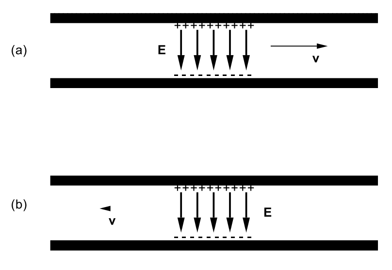
the other electrode as shown schematically in Figure (11.4.7). The charge patches move down the line with the velocity v characteristic of the wave velocity in the medium between the electrodes. At any section of the line the current on either electrode is zero until the charge patch arrives. Current is the rate at which charge is transported past a particular point, therefore the current at some point on the electrode is the product of the velocity and the charge density per unit length of line. It is clear from Figure (11.4.7(a)), which depicts a positive voltage pulse moving to the right, that the current in the upper electrode will be positive, whereas the current pulse carried by the lower electrode will be negative because negative charge is flowing from left to right. Similarly, if the pulse is moving from right to left the current flow in the upper conductor will be negative because positive charges are flowing in the negative z direction. At the same time, the current in the bottom electrode is positive because negative charges are flowing from right to left. For a positive voltage pulse moving from left to right one adopts the convention that the associated current pulse is positive. For a positive voltage pulse moving from right to left one adopts the convention that the associated current pulse is negative.