
11.6: Sinusoidal Signals on a Terminated Line


- Last updated
- Jun 21, 2021
- Save as PDF

( \newcommand{\kernel}{\mathrm{null}\,}\)
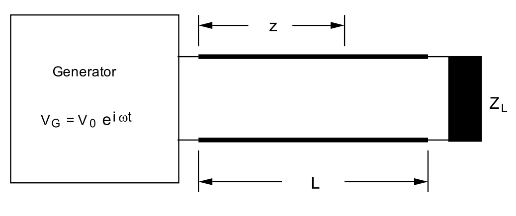
Let a transmission line having a characteristic impedance Z0 be used to connect a sinusoidal signal generator to a load, ZL, as shown in Figure (11.6.12). In phasor notation the generator voltage may be written
VG(t)=V0exp[iωt];
this corresponds to a real time variation cos ωt. A positive sign has been used in the phasor exponential in accord with the usual engineering convention for the description of alternating current circuits. The potential difference at any point along the line will consist of a forward propagating wave plus a backward propagating wave due to a reflection from the load. Recall that the current and potential waves must be functions of (z-vt) and (z+vt) in order to satisfy Maxwell’s equations (11.3.8). The forward propagating voltage wave
must therefore have the form
Vf(z,t)=aexp(−iωv[z−vt])=aexp(−iωzv)exp(iωt),
and the reflected wave must have the form
Vr(z,t)=bexp(iωv[z+vt])=bexp(iωZv)exp(iωt),
where a,b are constants that must be determined from the generator potential and from the boundary conditions at the load, i.e. ZL = V/I. It is customary to write k = ω/v, where ω = 2πf and where v is the velocity of a pulse on the cable. The potential difference at any point along the line is given by
V(z,t)=(aexp(−ikz)+bexp(+ikz))exp(+iωt),
and the current is given by
I(z,t)=((aZ0)exp(−ikz)−(bZ0)exp(+ikz))exp(+iωt).
The expression (???) for the current follows from Equation (???) for the voltage combined with the transmission line characteristic impedances for forward and backward propagating waves, Equations (11.2.8) and (11.2.9). At the generator, assumed to be located at z=0, one has
V0=a+b.
At the load, assumed to be at z=L, one has
V/I=ZL,
or
(aexp(−ikL)+bexp(+ikL)aexp(−ikL)−bexp(+ikL))=(ZLZ0).
The above two equations can be solved to give
a=(zLZ0+1)V0((zLZ0+1)+(zLZ0−1)exp(−2ikL))b=(ZLZ0−1)V0exp(−2ikL)((ZLZ0+1)+(ZLZ0−1)exp(−2ikL)).
The impedance as seen by the generator can be obtained from the voltage and the current at z=0:
ZG=V(z=0)I(z=0)=V0[a−b]Z0,
or
ZGZ0=(zLZ0+1)+(ZLZ0−1)exp(−2ikL)((zLZ0+1)−(ZLZ0−1)exp(−2ikL)).
Or, introducing the reduced impedance zG = ZL/Z0 and the new variable Γ, where
Γ=(ZLZ0−1ZLZ0+1)=(zL−1zL+1),
one finds
zG=(1+Γexp(−2ikL)1−Γexp(−2ikL))=(exp(+ikL)+Γexp(−ikL)exp(+ikL)−Γexp(−ikL)).
In the above development it has been assumed that the cable is lossless.
The expression for the load on the generator, Equation (???), is rather complicated but it should be clear that the impedance as seen from the generator may be quite different from the load impedance especially if the length of the cable, L, is comparable to, or larger than, the wavelength of the disturbance on the cable, λ, where
k=2πλ=ω/v.
A few concrete examples may help to form a picture of how a cable can be used to transform a load impedance.
11.6.1 Case(1). A Shorted Cable.
For this case ZL = 0 and Γ= -1 from Equation (???) so that
First of all, notice that the impedance as seen from the generator is not in general equal to zero: in fact, when the cable length is such that kL=π/2, 3π/2, 5π/2, etc. the generator appears to be attached to an open circuit! If cable losses are taken into account (see below), the load on the generator will be finite at these lengths but large compared with the characteristic impedance providing that the line is not too long. The condition kL=π/2 corresponds to a cable that is a quarter wavelength long, L=λ/4. Secondly, if the impedance as seen from the generator is not zero (i.e. L not a multiple of a half-wavelength) or infinite (L an odd multiple of a quarter wavelength) it appears to be a pure reactance if the cable is lossless. This makes sense since a lossless cable and a lossless load cannot absorb any energy from the generator. For example, if kL=π/4, L=λ/8, the impedance at the generator is ZG = +iZ0, and therefore the generator looks into a purely inductive load.
11.6.2 Case(2). An Open-ended Cable.
For this case ZL = ∞ and therefore Γ = +1 from Equation (???). The reduced impedance at the generator terminals is given by
zG=1+exp(−2ikL)1−exp(−2ikL)=−icotkL.
The generator load appears to be an open circuit if the length of the cable is a multiple of a half-wavelength. A cable whose length is an odd multiple of a quarter wavelength presents a short circuit to the generator. For other cable lengths the generator would appear to be connected to a capacitor or an inductor according to whether cot kL was positive or negative.
11.6.3 Case(3). The Cable is Terminated by the Characteristic Impedance.
For this case Γ = 0 from Equation (???) and therefore the impedance at the generator is zG = 1, or ZG = Z0. The load across the generator is independent of the length of the cable.
11.6.4 Case(4). A Purely Inductive Load.
Let the inductor be such that ZL = iLω is equal in magnitude to the characteristic impedance, Z0. Then zL = ZL/Z0 and therefore
Γ=i−1i+1=+i.
The normalized load on the generator, from Equation (???), is
zG=ZGZ0=(1+sin2kL+icos2kL1−sin2kL−icos2kL).
In the limit as kL → π/4 (L→ λ/8) the generator appears to be attached to an open circuit. However, for a quarter wavelength line, kL = π/2, the generator load appears to be due to a pure capacitance such that 1/Cω = Z0. For kL=3π/4, L = 3λ/8, the generator looks into a short circuit. Finally for a half-wavelength cable the generator sees a an inductive reactance such that Lω = Z0. As the cable length is increased further the whole cycle is repeated.
11.6.5 Case(5). A Purely Capacitive Load.
Let the capacitor be such that ZL = −i/Cω has the magnitude of the characteristic impedance, Z0. For this case zL = ZL/Z0 = −i, and
Γ=zL−1zL+1=−i.
The normalized impedance as seen by the generator is given by
zG=ZGZ0=(1−sin2kL−icos2kL1+sin2kL+icos2kL).
This case is very similar to that of the cable terminated by an inductor. For kL=π/4, L=λ/8, the generator is short circuited because zG = 0. For a quarter wavelength line, kL=π/2, the generator looks into a pure inductance, zG= +i. For kL=3π/4, L=3λ/8, one finds that zG → ∞ so that the generator appears to be looking into an open circuit. Finally, for a half-wavelength line, kL=π, the same effect is obtained as if the load were connected directly across the generator. The whole cycle is repeated as the cable length is increased.
11.6.6 Summary
The following conclusions can be drawn from the above examples:
- A cable acts like an impedance transformer.
- A lossless cable whose length is an integral number of half-wavelengths long effectively places the load directly across the generator terminals, i.e. ZG = ZL.
- A lossless cable whose length is an odd multiple of a quarter wavelength acts like an impedance inverter. For this case exp (−2ikL) = −1 so that from Equation (???)
zG=1−Γ1+Γ≡1/zL.
The formula for the impedance at the generator terminals in terms of the load impedance and the length of the cable that connects the load to the generator, Equation (???), is very complicated. Graphical methods have been developed for determining the load on the generator given the load impedance, ZL, and the characteristics of the transmission line. A very common method is based on the use of a Smith chart: it is described in detail in the book ”Microwave Measurements” by E.L.Ginzton, McGraw-Hill, New York, 1957; section 4.9. The need for a graphical technique has become very much less pressing now that digital computers have become readily available.