3.10: A Geophysical Example
- Page ID
- 5767
\( \newcommand{\vecs}[1]{\overset { \scriptstyle \rightharpoonup} {\mathbf{#1}} } \)
\( \newcommand{\vecd}[1]{\overset{-\!-\!\rightharpoonup}{\vphantom{a}\smash {#1}}} \)
\( \newcommand{\id}{\mathrm{id}}\) \( \newcommand{\Span}{\mathrm{span}}\)
( \newcommand{\kernel}{\mathrm{null}\,}\) \( \newcommand{\range}{\mathrm{range}\,}\)
\( \newcommand{\RealPart}{\mathrm{Re}}\) \( \newcommand{\ImaginaryPart}{\mathrm{Im}}\)
\( \newcommand{\Argument}{\mathrm{Arg}}\) \( \newcommand{\norm}[1]{\| #1 \|}\)
\( \newcommand{\inner}[2]{\langle #1, #2 \rangle}\)
\( \newcommand{\Span}{\mathrm{span}}\)
\( \newcommand{\id}{\mathrm{id}}\)
\( \newcommand{\Span}{\mathrm{span}}\)
\( \newcommand{\kernel}{\mathrm{null}\,}\)
\( \newcommand{\range}{\mathrm{range}\,}\)
\( \newcommand{\RealPart}{\mathrm{Re}}\)
\( \newcommand{\ImaginaryPart}{\mathrm{Im}}\)
\( \newcommand{\Argument}{\mathrm{Arg}}\)
\( \newcommand{\norm}[1]{\| #1 \|}\)
\( \newcommand{\inner}[2]{\langle #1, #2 \rangle}\)
\( \newcommand{\Span}{\mathrm{span}}\) \( \newcommand{\AA}{\unicode[.8,0]{x212B}}\)
\( \newcommand{\vectorA}[1]{\vec{#1}} % arrow\)
\( \newcommand{\vectorAt}[1]{\vec{\text{#1}}} % arrow\)
\( \newcommand{\vectorB}[1]{\overset { \scriptstyle \rightharpoonup} {\mathbf{#1}} } \)
\( \newcommand{\vectorC}[1]{\textbf{#1}} \)
\( \newcommand{\vectorD}[1]{\overrightarrow{#1}} \)
\( \newcommand{\vectorDt}[1]{\overrightarrow{\text{#1}}} \)
\( \newcommand{\vectE}[1]{\overset{-\!-\!\rightharpoonup}{\vphantom{a}\smash{\mathbf {#1}}}} \)
\( \newcommand{\vecs}[1]{\overset { \scriptstyle \rightharpoonup} {\mathbf{#1}} } \)
\( \newcommand{\vecd}[1]{\overset{-\!-\!\rightharpoonup}{\vphantom{a}\smash {#1}}} \)
\(\newcommand{\avec}{\mathbf a}\) \(\newcommand{\bvec}{\mathbf b}\) \(\newcommand{\cvec}{\mathbf c}\) \(\newcommand{\dvec}{\mathbf d}\) \(\newcommand{\dtil}{\widetilde{\mathbf d}}\) \(\newcommand{\evec}{\mathbf e}\) \(\newcommand{\fvec}{\mathbf f}\) \(\newcommand{\nvec}{\mathbf n}\) \(\newcommand{\pvec}{\mathbf p}\) \(\newcommand{\qvec}{\mathbf q}\) \(\newcommand{\svec}{\mathbf s}\) \(\newcommand{\tvec}{\mathbf t}\) \(\newcommand{\uvec}{\mathbf u}\) \(\newcommand{\vvec}{\mathbf v}\) \(\newcommand{\wvec}{\mathbf w}\) \(\newcommand{\xvec}{\mathbf x}\) \(\newcommand{\yvec}{\mathbf y}\) \(\newcommand{\zvec}{\mathbf z}\) \(\newcommand{\rvec}{\mathbf r}\) \(\newcommand{\mvec}{\mathbf m}\) \(\newcommand{\zerovec}{\mathbf 0}\) \(\newcommand{\onevec}{\mathbf 1}\) \(\newcommand{\real}{\mathbb R}\) \(\newcommand{\twovec}[2]{\left[\begin{array}{r}#1 \\ #2 \end{array}\right]}\) \(\newcommand{\ctwovec}[2]{\left[\begin{array}{c}#1 \\ #2 \end{array}\right]}\) \(\newcommand{\threevec}[3]{\left[\begin{array}{r}#1 \\ #2 \\ #3 \end{array}\right]}\) \(\newcommand{\cthreevec}[3]{\left[\begin{array}{c}#1 \\ #2 \\ #3 \end{array}\right]}\) \(\newcommand{\fourvec}[4]{\left[\begin{array}{r}#1 \\ #2 \\ #3 \\ #4 \end{array}\right]}\) \(\newcommand{\cfourvec}[4]{\left[\begin{array}{c}#1 \\ #2 \\ #3 \\ #4 \end{array}\right]}\) \(\newcommand{\fivevec}[5]{\left[\begin{array}{r}#1 \\ #2 \\ #3 \\ #4 \\ #5 \\ \end{array}\right]}\) \(\newcommand{\cfivevec}[5]{\left[\begin{array}{c}#1 \\ #2 \\ #3 \\ #4 \\ #5 \\ \end{array}\right]}\) \(\newcommand{\mattwo}[4]{\left[\begin{array}{rr}#1 \amp #2 \\ #3 \amp #4 \\ \end{array}\right]}\) \(\newcommand{\laspan}[1]{\text{Span}\{#1\}}\) \(\newcommand{\bcal}{\cal B}\) \(\newcommand{\ccal}{\cal C}\) \(\newcommand{\scal}{\cal S}\) \(\newcommand{\wcal}{\cal W}\) \(\newcommand{\ecal}{\cal E}\) \(\newcommand{\coords}[2]{\left\{#1\right\}_{#2}}\) \(\newcommand{\gray}[1]{\color{gray}{#1}}\) \(\newcommand{\lgray}[1]{\color{lightgray}{#1}}\) \(\newcommand{\rank}{\operatorname{rank}}\) \(\newcommand{\row}{\text{Row}}\) \(\newcommand{\col}{\text{Col}}\) \(\renewcommand{\row}{\text{Row}}\) \(\newcommand{\nul}{\text{Nul}}\) \(\newcommand{\var}{\text{Var}}\) \(\newcommand{\corr}{\text{corr}}\) \(\newcommand{\len}[1]{\left|#1\right|}\) \(\newcommand{\bbar}{\overline{\bvec}}\) \(\newcommand{\bhat}{\widehat{\bvec}}\) \(\newcommand{\bperp}{\bvec^\perp}\) \(\newcommand{\xhat}{\widehat{\xvec}}\) \(\newcommand{\vhat}{\widehat{\vvec}}\) \(\newcommand{\uhat}{\widehat{\uvec}}\) \(\newcommand{\what}{\widehat{\wvec}}\) \(\newcommand{\Sighat}{\widehat{\Sigma}}\) \(\newcommand{\lt}{<}\) \(\newcommand{\gt}{>}\) \(\newcommand{\amp}{&}\) \(\definecolor{fillinmathshade}{gray}{0.9}\)Assume that planet Earth is spherical and that it has a little magnet or current loop at its centre. By “little” I mean small compared with the radius of the Earth. Suppose that, at a large distance from the magnet or current loop the geometry of the magnetic field is the same as that of an electric field at a large distance from a simple dipole. That is to say, the equation to the lines of force is
\[r=a\sin^2 \theta \]
and the differential equation to the lines of force is
\[\frac{dr}{dθ} = \frac{2r}{tan \theta}\]
Show that the angle of dip \(D\) at geomagnetic latitude \(L\) is given by
\[\tan D = 2\tan L \label{3.10.1}\]
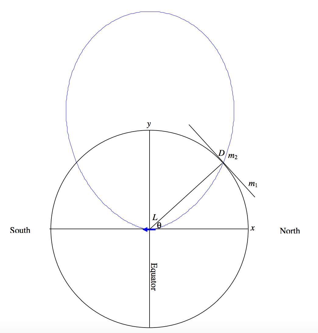
The geometry is shown in Figure \(III\).16.
The result is a simple one, and there is probably a simpler way of getting it than the one I tried. Let me know (jtatum@uvic.ca) if you find a simpler way. In the meantime, here is my solution.
I am going to try to find the slope \(m_1\) of the tangent to Earth (i.e. of the horizon) and the slope \(m_2\) of the line of force. Then the angle D between them will be given by the equation (which I am hoping is well known from coordinate geometry!)
\[\tan D = \frac{m_1 -m_2}{1+m_1m_2}. \label{3.10.2}\]
The first is easy:
\[m_1=\tan (90^\circ + \theta ) = -\frac{1}{\tan \theta}\label{3.10.3}\]
For \(m_2\) we want to find the slope of the line of force, whose equation is given in polar coordinates. So, how do you find the slope of a curve whose equation is given in polar coordinates? We can do it like this:
\[\begin{align} x&=r\cos \theta \label{3.10.4}, \\ y&=r\sin \theta \label{3.10.5}, \\ dx&=\cos \theta dr - r\sin \theta d\theta \label{3.10.6}, \\ dy&=\sin \theta dr + r\cos \theta d\theta . \label{3.10.7} \\ \end{align}\]
From these, we obtain
\[\frac{dy}{dx}=\frac{\sin \theta \frac{dr}{d\theta}+r\cos \theta }{\cos \theta \frac{dr}{d\theta}-r\sin \theta }.\label{3.10.8} \]
In our particular case, we have \(\frac{dr}{d\theta}=\frac{2r}{\tan \theta}\) (equation 3.7.12), so if we substitute this into Equation \(\ref{3.10.8}\) we soon obtain
\[m_2 = \frac{3\sin \theta \cos \theta}{3\cos^2 \theta -1}.\label{3.10.9} \]
Now put Equations \ref{3.10.3} and \ref{3.10.9} into equation 3.10.2, and, after a little algebra, we soon obtain
\[\tan D = \frac{2}{\tan \theta}=2\tan L . \label{3.10.10}\]
Here is another question. The magnetic field is generally given the symbol \(B\). Show that the strength of the magnetic field \(B(L)\) at geomagnetic latitude \(L\) is given by
\[B(L) = B(0)\sqrt{1+3\sin^2 L } ,\label{3.10.11} \]
where \(B(0)\) is the strength of the field at the equator. This means that it is twice as strong at the magnetic poles as at the equator.
Start with equation 3.7.2, which gives the electric field at a distant point on the equator of an electric dipole. That equation was \(E=\frac{p}{4\pi\epsilon_0 y^3}\). In this case we are dealing with a magnetic field and a magnetic dipole, so we’ll replace the electric field \(E\) with a magnetic field \(B\). Also \(p/(4π\epsilon_0)\) is a combination of electrical quantities, and since we are interested only in the geometry (i.e. on how \(B\) varies from equation to pole, let’s just write \(p/(4\pi\epsilon_0 )\) as \(k\). And we’ll take the radius of Earth to be \(R\), so that equation 3.7.2 gives for the magnetic field at the surface of Earth on the equator as
\[B(0) = \frac{k}{R^3}. \label{3.10.12} \]
In a similar vein, equations 3.7.10 for the radial and transverse components of the field at geomagnetic latitude \(L\) (which is 90º − \(θ\)) become
\[B_r ( L) = \frac{2k\sin L}{R^3} \quad \text{and} \quad B_{\theta}(L)=\frac{k\cos L}{R^3}. \label{3.10.13a,b}\]
And since \(B=\sqrt{B_r^2 + B_{\theta}^2}\) the result immediately follows.