3.9: Potential at a Large Distance from a Charged Body

We wish to find the potential at a point P at a large distance $R$ from a charged body, in terms of its total charge and its dipole, quadrupole, and possibly higher-order moments. There will be no loss of generality if we choose a set of axes such that P is on the $z$-axis.

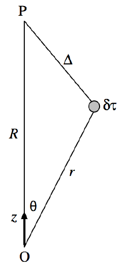
$\text{FIGURE III.14}$

We refer to Figure $III$.14, and we consider a volume element $δτ$ at a distance r from some origin. The point P is at a distance r from the origin and a distance $∆ \text{ from }δτ$. The potential at P from the charge in the element $δτ$ is given by

$$4\pi\epsilon_0 \delta V = \dfrac{\rho \delta \tau }{\Delta} = \dfrac{\rho}{R}\left ( 1+\dfrac{r^2}{R^2}-\dfrac{2r}{R}\cos \theta \right )^{-1/2}\delta \tau ,$$

and so the potential from the charge on the whole body is given by

$$4\pi\epsilon_0 V =\dfrac{1}{R} \int \rho \left ( 1+\dfrac{r^2}{R^2} -\dfrac{2r}{R}\cos \theta \right )^{-1/2}\delta \tau .$$

On expanding the parentheses by the binomial theorem, we find, after a little trouble, that this becomes

$$4\pi\epsilon_0 V = \dfrac{1}{R}\int \rho \,d\tau + \dfrac{1}{R^2}\int \rho r P_1 (\cos \theta)\,d\tau + \dfrac{1}{2!R^3}\int \rho r^2 P_2 (\cos \theta)]\, d\tau + \dfrac{1}{3!R^4}\int \rho r^3 P_3 (\cos \theta )\,d\tau + ... ,$$

where the polynomials P are the Legendre polynomials given by

$$\begin{align}P_1 (\cos \theta ) &= \cos \theta \\ P_2(\cos \theta) &= \dfrac{1}{2}(3\cos^2 \theta -1 ), \\ P_3(\cos \theta)&=\dfrac{1}{2}(5\cos^3 \theta - 3\cos \theta ). \\ \end{align}$$

We see from the forms of these integrals and the definitions of the components of the dipole and quadrupole moments that this can now be written:

$$4\pi\epsilon_0 V = \dfrac{Q}{R} + \dfrac{p}{R^2}+\dfrac{1}{2R^3}(3q_{zz}-Tr\textbf{q})+...,\label{3.9.7}$$

Here Tr q is the trace of the quadrupole moment matrix, or the (invariant) sum of its diagonal elements. Equation $\ref{3.9.7}$ can also be written

$$4\pi\epsilon_0V=\dfrac{Q}{R}+\dfrac{p}{R^2}+\dfrac{1}{2R^3}[2q_{zz}-(q_{xx}+q_{yy})]+... .$$

The quantity $2q_{zz}-(q_{xx}+q_{yy})$ of the diagonalized matrix is often referred to as “the” quadrupole moment. It is zero if all three diagonal components are zero or if $q_{zz}=\dfrac{1}{2}(q_{xx}+q_{yy})$. If the body has cylindrical symmetry about the $z$-axis, this becomes $2(q_{zz}-q_{xx})$.

.)

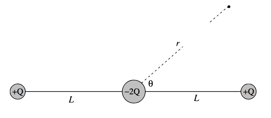
$\text{FIGURE III.15}$

The solution to this exercise is easy if you know about Legendre polynomials. See Section 1.14 of my notes on Celestial Mechanics. What you need to know is that the expansion of $(1-2ax+x^2)^{-1/2}$ can be written as a series of Legendre polynomials, namely $P_0(x)+xP_1(x)+x^2P_2(x)+...$. You also need a (very small) table of Legendre polynamials, namely $P_0(x)=1,\,P_1(x)=x,\,P_2(x)=\dfrac{1}{2}(3x^2-1)$. Given that, you should find the exercise very easy.