2.5: Capacitance

Let us start using the macroscopic model from systems consisting of charged conductors only, with no so-called stand-alone charges in the free space outside them.¹¹ Our goal here is to calculate the distributions of the electric field \(\ \mathbf{E}\) and potential \(\ \phi\) in space, and the distribution of the surface charge density \(\ \sigma\) over the conductor surfaces. However, before doing that for particular situations, let us see if there are any integral measures of these distributions, that should be our primary focus.

The simplest case is of course a single conductor in the otherwise free space. According to Eq. (1b), all its volume should have the same electrostatic potential \(\ \phi\), evidently providing one convenient global measure of the situation. Another integral measure is provided by the total charge

\[\ Q \equiv \int_{V} \rho d^{3} r \equiv \oint_{S} \sigma d^{2} r,\tag{2.11}\]

where the latter integral is extended over the whole surface S of the conductor. In the general case, what we can tell about the relation between \(\ Q\) and \(\ \phi\)? At \(\ Q=0\), there is no electric field in the system, and it is natural (though not absolutely necessary) to select the arbitrary constant in the electrostatic potential to have \(\ \phi=0\) everywhere. Then, if the conductor is charged with a non-zero \(\ Q\), according to the linear Eq. (1.7), the electric field in any point of space has to be proportional to that charge. Hence the electrostatic potential at all points, including its value \(\ \phi\) inside the conductor, is also proportional to \(\ Q\):

\[\ \phi=p Q.\tag{2.12}\]

The proportionality coefficient \(\ p\), which depends on the conductor’s size and shape, but neither on \(\ \phi\) nor on \(\ Q\), is called the reciprocal capacitance (or, not too often, “electric elastance”). Usually, Eq. (12) is rewritten in a different form,

Self-capacitance

\[\ Q=C \phi, \quad \text { with } C \equiv \frac{1}{p},\tag{2.13}\]

where \(\ C\) is called self-capacitance. (Frequently, C is called just capacitance, but as we will see very soon, for more complex situations the latter term may be ambiguous.)

Before calculating \(\ C\) for particular geometries, let us have a look at the electrostatic energy \(\ U\) of a single conductor. To calculate it, of the several relations discussed in Chapter 1, Eq. (1.61) is most convenient, because all elementary charges \(\ q_{k}\) are now parts of the conductor charge, and hence reside at the same potential \(\ \phi\) - see Eq. (1b) again. As a result, the equality becomes very simple:

\[\ U=\frac{1}{2} \phi \sum_{k} q_{k} \equiv \frac{1}{2} \phi Q.\tag{2.14}\]

Moreover, using the linear relation (13), the same result may be re-written in two more forms:

Electro-static energy

\[\ U=\frac{Q^{2}}{2 C}=\frac{C}{2} \phi^{2}.\tag{2.15}\]

We will discuss several ways to calculate \(\ C\) in the next sections, and right now will have a quick look at just the simplest example for which we have calculated everything necessary in the previous chapter: a conducting sphere of radius \(\ R\). Indeed, we already know the electric field distribution: according to Eq. (1), \(\ E=0\) inside the sphere, while Eq. (1.19), with \(\ Q(r)=Q\), describes the field distribution outside it, because of the evident spherical symmetry of the surface charge distribution. Moreover, since the latter formula is exactly the same as for the point charge placed in the sphere’s center, the potential’s distribution in space can be obtained from Eq. (1.35) by replacing \(\ q\) with the sphere’s full charge \(\ Q\). Hence, on the surface of the sphere (and, according to Eq. (1b), through its
interior),

\[\ \phi=\frac{1}{4 \pi \varepsilon_{0}} \frac{Q}{R}.\tag{2.16}\]

Comparing this result with the definition (13), for the self-capacitance we obtain a very simple formula

\[\ C=4 \pi \varepsilon_{0} R.\tag{2.17}\]

This formula, which should be well familiar to the reader,¹² is convenient to get some feeling of how large the SI unit of capacitance (1 farad, abbreviated as F) is: the self-capacitance of Earth \(\ (R_{\mathrm{E}} \approx6.34\times10^6\text{m})\) is below 1 mF! Another important note is that while Eq. (17) is not exactly valid for a
conductor of arbitrary shape, it implies an important general estimate

\[\ C \sim 2 \pi \varepsilon_{0} a\tag{2.18}\]

where \(\ a\) is the scale of the linear size of any conductor.¹³

Now proceeding to a system of two arbitrary conductors, we immediately see why we should be careful with the capacitance definition: one constant \(\ C\) is insufficient to describe such a system. Indeed, here we have two, generally different conductor potentials, \(\ \phi_{1}\) and \(\ \phi_{2}\), that may depend on both conductor charges, \(\ Q_{1}\) and \(\ Q_{2}\). Using the same arguments as for the single-conductor case, we may conclude that the dependence is always linear:

\[\ \begin{aligned}
&\phi_{1}=p_{11} Q_{1}+p_{12} Q_{2}, \\
&\phi_{2}=p_{21} Q_{1}+p_{22} Q_{2},
\end{aligned}\tag{2.19}\]

but now has to be described by more than one coefficient. Actually, it turns out that there are three rather than four different coefficients in these relations, because

\[\ p_{12}=p_{21}.\tag{2.20}\]

This equality may be proved in several ways, for example, using the general reciprocity theorem of electrostatics (whose proof was the subject of Problem 1.17):

\[\ \int \rho_{1}(\mathbf{r}) \phi^{(2)}(\mathbf{r}) d^{3} r=\int \rho_{2}(\mathbf{r}) \phi^{(1)}(\mathbf{r}) d^{3}r,\tag{2.21}\]

where \(\ \phi^{(1)}(\mathbf{r})\) and \(\ \phi^{(2)}(\mathbf{r})\) are the potential distributions induced, respectively, by two electric charge distributions, \(\ \rho_{1}(\mathbf{r})\) and \(\ \rho_{2}(\mathbf{r})\). In our current case, each of these integrals is limited to the volume (or, more exactly, the surface) of the corresponding conductor, where each potential is constant and may be taken out of the integral. As a result, Eq. (21) is reduced to

\[\ Q_{1} \phi^{(2)}\left(\mathbf{r}_{1}\right)=Q_{2} \phi^{(1)}\left(\mathbf{r}_{2}\right).\tag{2.22}\]

In terms of Eq. (19), \(\ \phi^{(2)}\left(\mathbf{r}_{1}\right)\) is just \(\ p_{12} Q_{2}\), while \(\ \phi^{(1)}\left(\mathbf{r}_{2}\right)\) equals \(\ p_{21} Q_{1}\). Plugging these expressions into Eq. (22), and canceling the products \(\ Q_{1} Q_{2}\), we arrive at Eq. (20).

Hence the 2x2 matrix of coefficients \(\ p_{jj}\), (called the reciprocal capacitance matrix) is always symmetric, and using the natural notation \(\ p_{11} \equiv p_{1}, p_{22} \equiv p_{2}, p_{12}=p_{21} \equiv p\), we may rewrite it in a simpler form:

\[\ \left(\begin{array}{ll}
p_{1} & p \\
p & p_{2}
\end{array}\right).\tag{2.23}\]

Plugging the relation (19), in this new notation, into Eq. (1.61), we see that the full electrostatic energy of the system may be expressed as a quadratic form of its charges:

\[\ U=\frac{p_{1}}{2} Q_{1}^{2}+p Q_{1} Q_{2}+\frac{p_{2}}{2} Q_{2}^{2}.\tag{2.24}\]

It is evident that the middle term on the right-hand side of this equation describes the electrostatic coupling of the conductors. (Without it, the energy would be just a sum of two independent electrostatic energies of conductors 1 and 2.)¹⁴ Still, even with this simplification, Eqs. (19) and (20) show that in the general case of arbitrary charges \(\ Q_{1}\) and \(\ Q_{2}\), the system of two conductors should be characterized by three, rather than just one coefficient (“the capacitance”). This is why we may attribute a certain single capacitance to the system only in some particular cases.

For practice, the most important of them is when the system as the whole is electrically neutral: \(\ Q_{1}=-Q_{2} \equiv Q\). In this case, the most important function of Q is the difference of the conductors’ potentials, called the voltage:¹⁵

Voltage: definition

\[\ V \equiv \phi_{1}-\phi_{2},\tag{2.25}\]

For that function, the subtraction of two Eqs. (19) gives

Mutual capacitance

\[\ V=\frac{Q}{C}, \quad \text { with } C \equiv \frac{1}{p_{1}+p_{2}-2 p},\tag{2.26}\]

where the coefficient \(\ C\) is called the mutual capacitance between the conductors – or, again, just “capacitance”, if the term’s meaning is absolutely clear from the context. The same coefficient describes the electrostatic energy of the system. Indeed, plugging Eqs. (19) and (20) into Eq. (24), we see that both forms of Eq. (15) are reproduced if \(\ \phi\) is replaced with \(\ V\), \(\ Q_{1}\) with \(\ Q\), and with \(\ C\) meaning the mutual capacitance:

Capacitor’s energy

\[\ U=\frac{Q^{2}}{2 C}=\frac{C}{2} V^{2}.\tag{2.27}\]

The best-known system for which the mutual capacitance \(\ C\) may be readily calculated is the plane (or “parallel-plate”) capacitor, a system of two conductors separated with a narrow plane gap of a constant thickness \(\ d\) and an area \(\ A \sim a^{2} \gg d^{2}\) – see Fig. 3.

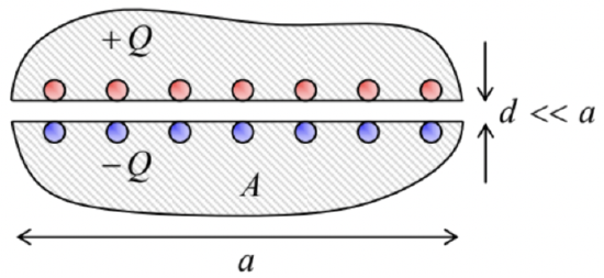Fig. 2.3. Plane capacitor – schematically.

Since the surface charges, that contribute to the opposite charges \(\ \pm Q\) of the conductors of this system, attract each other, in the limit \(\ d<<a\) they sit entirely on the opposite surfaces limiting the gap, so there is virtually no electric field outside of the gap, while (according to the discussion in Sec. 1) inside the gap it is normal to the surfaces. According to Eq. (3), the magnitude of this field is \(\ E=\sigma / \varepsilon_{0}\). Integrating this field across thickness \(\ d\) of the narrow gap, we get \(\ V \equiv \phi_{1}-\phi_{2}=E d=\sigma d / \varepsilon_{0}\), so that \(\ \sigma=\varepsilon_{0} V / d\). But due to the constancy of the potential of each electrode, \(\ V\) should not depend on the position in the gap area. As a result, \(\ \sigma\) should be also constant over all the gap area \(\ A\), regardless of the external geometry of the conductors (see Fig. 3 again), and hence \(\ Q=\sigma A=\varepsilon_{0} V / d\). Thus we may write \(\ V=Q / C\), with

C: Plane capacitor

\[\ C=\frac{\varepsilon_{0} A}{d}.\tag{2.28}\]

Let me offer a few comments on this well-known formula. First, it is valid even if the gap is not quite planar – for example, if it gently curves on a scale much larger than \(\ d\), but retains its thickness. Second, Eq. (28), which is valid if \(\ A \sim a^{2}\) is much larger than \(\ d^{2}\), ignores the electric field deviations from uniformity¹⁶ at distances \(\ \sim d\) near the gap edges. Finally, the same condition \(\ \left(A \gg d^{2}\right)\) assures that \(\ C\) is much larger than the self-capacitance \(\ C_{j} \sim \varepsilon_{0} a\) of each conductor – see Eq. (18). The opportunities open by this fact for electronic engineering and experimental physics practice are rather astonishing. For example, a very realistic 3-nm layer of high-quality aluminum oxide (which may provide a nearly perfect electric insulation between two thin conducting films) with an area of \(\ 0.1 \mathrm{~m}^{2}\) (which is a typical area of silicon wafers used in the semiconductor industry) provides \(\ C \sim 1\),¹⁷ larger than the self-capacitance of the whole planet Earth!

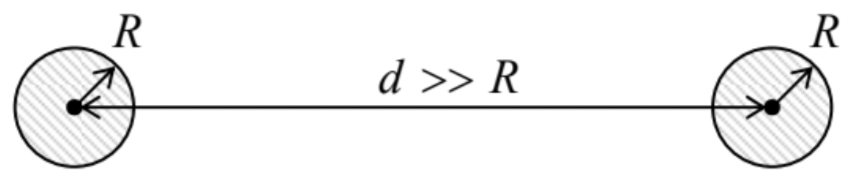
In the case shown in Fig. 3, the electrostatic coupling of the two conductors is evidently strong. As an opposite example of a weakly coupled system, let us consider two conducting spheres of the same radius \(\ R\), separated by a much larger distance \(\ d\) (Fig. 4).

Fig. 2.4. A system of two far separated, similar conducting spheres.

In this case, the diagonal components of the matrix (23) may be approximately found from Eq. (16), i.e. by neglecting the coupling altogether:

\[\ p_{1}=p_{2} \approx \frac{1}{4 \pi \varepsilon_{0} R}.\tag{2.29}\]

Now, if we had just one sphere (say, number 1), the electric potential at distance \(\ d\) from its center would be given by Eq. (16): \(\ \phi=Q_{1} / 4 \pi \varepsilon_{0} d\). If we move into this point a small \(\ (R<<d)\) sphere without its own charge, we may expect that its potential should not be too far from this result, so that \(\ \phi_{2} \approx Q_{1} / 4 \pi \varepsilon_{0} d\). Comparing this expression with the second of Eqs. (19) (taken for \(\ Q_{2}=0\)), we get

\[\ p \approx \frac{1}{4 \pi \varepsilon_{0} d}<<p_{1,2}.\tag{2.30}\]

From here and Eq. (26), the mutual capacitance

\[\ C \approx \frac{1}{p_{1}+p_{2}} \approx 2 \pi \varepsilon_{0} R.\tag{2.31}\]

We see that (somewhat counter-intuitively), in this limit \(\ C\) does not depend substantially on the distance between the spheres, i.e. does not describe their electrostatic coupling. The off-diagonal coefficients of the reciprocal capacitance matrix (20) play this role much better – see Eq. (30).

Now let us consider the case when only one conductor of the two is charged, for example \(\ Q_{1} \equiv Q\), while \(\ Q_{2}=0\). Then Eqs. (19)-(20) yield

\[\ \phi_{1}=p_{1} Q_{1}.\tag{2.32}\]

Now, we may follow Eq. (13) and define \(\ C_{1} \equiv 1 / p_{1}\) (and \(\ C_{2} \equiv 1 / p_{2}\)), just to see that such partial capacitances of the conductors of the system differ from its mutual capacitance \(\ C\) – cf. Eq. (26). For example, in the case shown in Fig. 4, \(\ C_{1}=C_{2} \approx 4 \pi \varepsilon_{0} R \approx 2 C\).

Finally, let us consider one more frequent case when one of the conductors carries a certain charge (say, \(\ Q_{1}=Q\)), but the potential of its counterpart is sustained constant, say \(\ \phi_{2}=0\).¹⁸ (This condition is especially easy to implement if the second conductor is much larger than the first one. Indeed, as the estimate (18) shows, in this case it would take a much larger charge \(\ Q_{2}\) to make the potential \(\ \phi_{2}\) comparable with \(\ \phi_{1}\).) In this case the second of Eqs. (19), with the account of Eq. (20), yields \(\ Q_{2}=-\left(p / p_{2}\right) Q_{1}\). Plugging this relation into the first of those equations, we get

\[\ Q_{1}=C_{1}^{\mathrm{ef}} \phi_{1}, \quad \text { with } C_{1}^{\mathrm{ef}} \equiv\left(p_{1}-\frac{p^{2}}{p_{2}}\right)^{-1} \equiv \frac{p_{2}}{p_{1} p_{2}-p^{2}}.\tag{2.33}\]

Thus, this effective capacitance of the first conductor is generally different both from both its partial capacitance \(\ C_{1}\) and the mutual capacitance \(\ C\) of the system, emphasizing again how accurate one should be using the term “capacitance” without a qualifier.

Note also that none of these capacitances is equal to any element of the matrix reciprocal to the matrix (23):

\[\ \left(\begin{array}{cc}
p_{1} & p \\
p & p_{2}
\end{array}\right)^{-1}=\frac{1}{p^{2}-p_{1} p_{2}}\left(\begin{array}{cc}
-p_{2} & p \\
p & -p_{1}
\end{array}\right).\tag{2.34}\]

Because of this reason, this physical capacitance matrix, which expresses the vector of conductor charges via the vector of their potentials, is less convenient for most applications than the reciprocal capacitance matrix (23). The same conclusion is valid for multi-conductor systems, which are most conveniently characterized by an evident generalization of Eq. (19). Indeed, in this case, even the mutual capacitance between two selected conductors may depend on the electrostatic conditions of other components of the system.

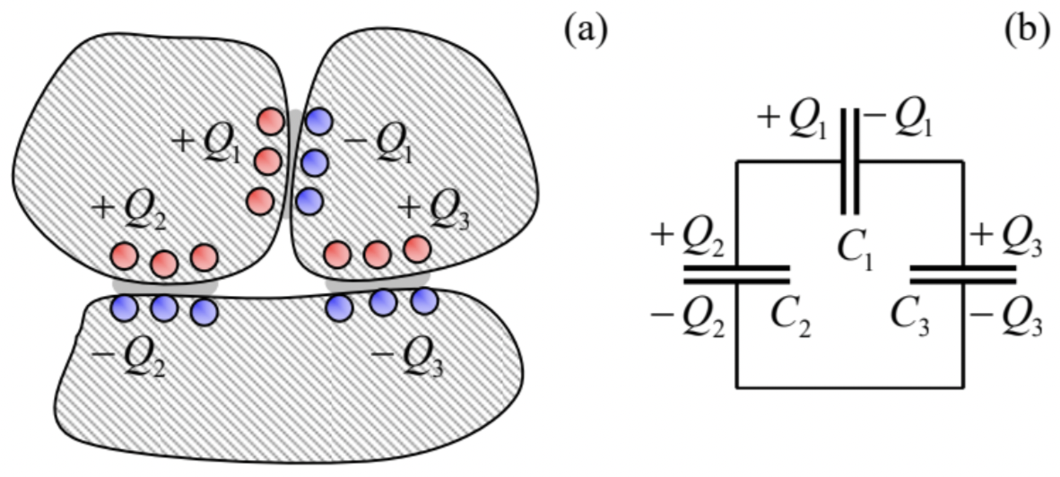
Logically, at this point I would need to discuss the particular, but practically very important case when the regions, where the electric field between each pair of conductors is most significant, do not overlap – such as in the example shown in Fig. 5a. In this case, the system’s properties may be discussed using the equivalent-circuit language, representing each such region as a lumped (localized) capacitor, with a certain mutual capacitance \(\ C\), and the whole system as some connection of these capacitors by conducting “wires”, whose length and geometry are not important – see Fig. 5b.

Fig. 2.5. (a) A simple system of conductors, with three well - localized regions of the electric field and surface charge concentration, and (b) its representation with an equivalent circuit of three lumped capacitors.

Since the analysis of such equivalent circuits is covered in typical introductory physics courses, I will save time by skipping their discussion. However, since such circuits are very frequently met in the physical experiment and electrical engineering practice, I would urge the reader to self-test their understanding of this topic by solving a couple of problems offered at the end of this chapter,¹⁹ and if their solution presents any difficulty, review the corresponding section in an undergraduate textbook.

---

Reference

¹¹ In some texts, these charges are called “free”. This term is somewhat misleading, because they may well be bound, i.e. unable to move freely.

¹² In the Gaussian units, using the standard replacement \(\ 4 \pi \varepsilon_{0} \rightarrow 1\), this relation takes an even simpler form: \(\ C = R\), very easy to remember. Generally, in the Gaussian units (but not in the SI system!) the capacitance has the dimensionality of length, i.e. is measured in centimeters. Note also that a fractional SI unit, 1 picofarad \(\ \left(10^{-12} \mathrm{~F}\right)\), is very close to the Gaussian unit: \(\ 1 \mathrm{pF}=\left(1 \times 10^{-12}\right) /\left(4 \pi \varepsilon_{0} \times 10^{-2}\right) \mathrm{cm} \approx 0.8998 \mathrm{~cm}\). So, 1 pF is close to the capacitance of a metallic ball with a 1-cm radius, making this unit very convenient for human-scale systems.

¹³ These arguments are somewhat insufficient to say which size should be used for \(\ a\) in the case of narrow, extended conductors, e.g., a thin, long wire. Very soon we will see that in such cases the electrostatic energy, and hence \(\ C\), depends mostly on the larger size of the conductor.

¹⁴ This is why systems with \(\ p<<p_{1}, p_{2}\) are called weakly coupled, and may be analyzed using approximate methods – see, e.g., Fig. 4 and its discussion below.

¹⁵ A word of caution: in condensed matter physics and electrical engineering, voltage is most often defined as the difference of electrochemical rather than electrostatic potentials. These two notions coincide if the conductors have equal workfunctions – for example, if they are made of the same material. In this course, this condition will be implied, and the difference between the two voltages ignored – to be discussed in detail in SM Sec. 6.3.

¹⁶ Such fringe fields result in an additional stray capacitance \(\ C^{\prime} \sim \varepsilon_{0} a<<C\sim \varepsilon_{0} a \times(a / d)\).

¹⁷ Just as in Sec. 1, for the estimate to be realistic, I took into account the additional factor \(\ K\) (for aluminum oxide, close to 10) which should be included in the numerator of Eq. (28) to make it applicable to dielectrics – see Chapter 3 below.

¹⁸ In electrical engineering, such a constant-potential conductor is called the ground. This term stems from the fact that in many cases the electrostatic potential of the (weakly) conducting ground at the Earth’s surface is virtually unaffected by laboratory-scale electric charges.

¹⁹ These problems have been selected to emphasize the fact that not every circuit may be reduced to the simplest connections of the capacitors in parallel and/or in series.