3.4: Electrostatics of Linear Dielectrics

First, let us discuss the simplest problem: how is the electrostatic field of a set of stand-alone charges of density \(\ \rho(\mathbf{r})\) modified by a uniform linear dielectric medium, which obeys Eq. (46) with a space-independent dielectric constant \(\ \kappa\). In this case, we may combine Eqs. (32) and (46) to write

\[\ \nabla \cdot \mathbf{E}=\frac{\rho}{\varepsilon}.\tag{3.53}\]

As a reminder, in the free space we had a similar equation (1.27), but with a different constant, \(\ \varepsilon_{0}=\varepsilon / \kappa\). Hence all the results discussed in Chapter 1 are valid inside a uniform linear dielectric, for the macroscopic field the \(\ \mathbf{E}\) (and the corresponding macroscopic electrostatic potential \(\ \phi\)), if they are reduced by the factor of \(\ \kappa>1\). Thus, the most straightforward result of the induced polarization of a dielectric medium is the electric field reduction. This is a very important effect, especially taken into account the very high values of \(\ \kappa\) in such dielectrics as water – see Table 1. Indeed, it is the reduction of the attraction between positive and negative ions (called, respectively, cations and anions) in water that enables their substantial dissociation and hence almost all biochemical reactions, which are the basis of the biological cell functions – and hence of the life itself.

Let us apply this general result to the important particular case of the plane capacitor (Fig. 2.3) filled with a linear, uniform dielectric. Applying the macroscopic Gauss law (34) to a pillbox-shaped volume on the conductor surface, we get the following relation,

\[\ \sigma=D_{n}=\varepsilon E_{n}=-\varepsilon \frac{\partial \phi}{\partial n},\tag{3.54}\]

which differs from Eq. (2.3) only by the replacement \(\ \varepsilon_{0} \rightarrow \varepsilon \equiv \kappa \varepsilon_{0}\). Hence, for a fixed field \(\ E_{n}\), the charge density calculated for the free-space case, should be increased by the factor of \(\ \kappa\) – that’s it. In particular, this means that the mutual capacitance (2.28) has to be increased by this factor:

C of a planar capacitor

\[\ C=\frac{\kappa \varepsilon_{0} A}{d} \equiv \frac{\varepsilon A}{d}.\tag{3.55}\]

(As a reminder, this increase of \(\ C\) by \(\ \kappa\) has been already incorporated, without derivation, into some estimates made in Secs. 2.1 and 2.2.)

If a linear dielectric is nonuniform, the situation is more complex. For example, let us consider the case of a sharp interface between two otherwise uniform dielectrics, free of stand-alone charges. In this case, we still may use Eq. (37) for the tangential component of the macroscopic electric field, and also Eq. (36), with \(\ D_{n}=\varepsilon E_{n}\), which yields

Boundary condition for \(\ E_{n}\)

\[\ \left(\varepsilon E_{n}\right)_{1}=\left(\varepsilon E_{n}\right)_{2}, \quad \text { i.e. } \varepsilon_{1} \frac{\partial \phi_{1}}{\partial n}=\varepsilon_{2} \frac{\partial \phi_{2}}{\partial n}.\tag{3.56}\]

Let us apply these boundary conditions, first of all, to the very illuminating case of two very thin \(\ (t<<d)\) slits carved in a uniform dielectric with an initially uniform²⁵ electric field \(\ \mathbf{E}_{0}\) (Fig. 9). In both cases, a slit with \(\ t \rightarrow 0\) cannot modify the field distribution outside it substantially.

Fig. 3.9. Fields inside two narrow slits cut in a linear dielectric with a uniform field \(\ \mathbf{E}_{0}\).

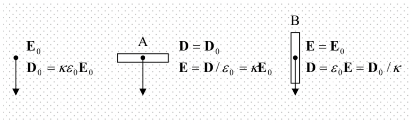
For slit A, with the plane normal to the applied field, we may apply Eq. (56) to the “major” (broad) interfaces, shown horizontal in Fig. 9, to see that the vector \(\ \mathbf { D }\) should be continuous. But according to Eq. (46), this means that in the free space inside the gap the electric field equals \(\ \mathbf{D} / \varepsilon_{0}\), and hence is \(\ \kappa\) times higher than the applied field \(\ \mathbf{E}_{0}=\mathbf{D} / \kappa \varepsilon_{0}\). This field, and hence \(\ \mathbf{D}\), may be measured by a sensor placed inside the gap, showing that the electric displacement is by no means a purely mathematical construct.²⁶ On the contrary, for the slit B parallel to the applied field, we may apply Eq. (37) to the major (now, vertical) interfaces of the slit, to see that now the electric field \(\ \mathbf{E}\) is continuous, while the electric displacement \(\ \mathbf{D}=\varepsilon_{0} \mathbf{E}\) inside the gap is a factor of \(\ \kappa\) lower than its value in the dielectric. (Similarly to case A, any perturbations of the field uniformity, caused by the compliance with Eq. (56) at the minor interfaces, settle down at distances ~t from them.)

For other problems with piecewise-constant \(\ \varepsilon\), with more complex geometries we may need to apply the methods studied in Chapter 2. As in the free space, in the simplest cases we can select such a set of orthogonal coordinates that the electrostatic potential depends on just one of them. Consider, for example, two types of plane capacitor’s filling with two different dielectrics – see Fig. 10.

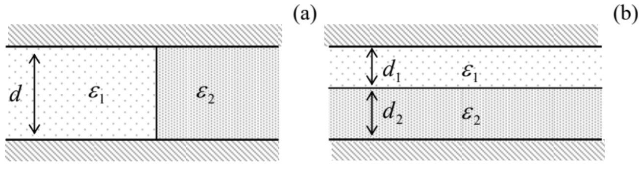Fig. 3.10. Plane capacitors filled with two different dielectrics.

In case (a), the voltage \(\ V\) between the electrodes is the same for each part of the capacitor, telling us that at least far from the dielectric interface, the electric field is vertical, uniform, and constant \(\ E=V / d\). Hence the boundary condition (37) is satisfied even if such a distribution is valid near the surface as well, i.e. at any point of the system. The only effect of different values of \(\ \varepsilon\) in the two parts is that the electric displacement \(\ D=\varepsilon E\) and hence electrodes’ surface charge density \(\ \sigma=D\) are different in the two parts. Thus we can calculate the electrode charges \(\ Q_{1,2}\) of the two parts independently, and then add up
the results to get the total mutual capacitance

\[\ C=\frac{Q_{1}+Q_{2}}{V}=\frac{1}{d}\left(\varepsilon_{1} A_{1}+\varepsilon_{2} A_{2}\right).\tag{3.57}\]

Note that this formula may be interpreted as the total capacitance of two separate lumped capacitors connected (by wires) in parallel. This is natural, because we may cut the system along the dielectric interface, without any effect on the fields in either part, and then connect the corresponding electrodes by external wires, again without any effect on the system – besides very close vicinities of capacitor’s edges.

Case (b) may be analyzed just as in the problem shown in Fig. 6, by applying Eq. (34) to a Gaussian pillbox with one lid inside the (for example) bottom electrode, and the other lid inside any of the layers. As a result, we see that \(\ D\) anywhere inside the system should be equal to the surface charge density \(\ \sigma\) of the electrode, i.e. constant. Hence, according to Eq. (46), the electric field inside each dielectric layer is also constant: in the top layer, it is \(\ E_{1}=D_{1} / \varepsilon_{1}=\sigma / \varepsilon_{1}\), while in bottom layer, \(\ E_{2}=D_{2} / \varepsilon_{2} = \sigma/\varepsilon_{2}\). Integrating the field \(\ E\) across the whole capacitor, we get

\[\ V=\int_{0}^{d_{1}+d_{2}} E(z) d z=E_{1} d_{1}+E_{2} d_{2}=\left(\frac{d_{1}}{\varepsilon_{1}}+\frac{d_{2}}{\varepsilon_{2}}\right) \sigma,\tag{3.58}\]

so that the mutual capacitance per unit area

\[\ \frac{C}{A} \equiv \frac{\sigma}{V}=\left[\frac{d_{1}}{\varepsilon_{1}}+\frac{d_{2}}{\varepsilon_{2}}\right]^{-1}.\tag{3.59}\]

Note that this result is similar to the total capacitance of an in-series connection of two plane capacitors based on each of the layers. This is also natural because we could insert an uncharged, thin conducting sheet (rather than a cut as in the previous case) at the layer interface, which is an equipotential surface, without changing the field distribution in any part of the system. Then we could thicken the conducting sheet as much as we like (and possibly shaping its internal part into a wire), also without changing the fields in the dielectric parts of the system, and hence its capacitance.

Proceeding to problems with more complex geometry, let us consider the system shown in Fig.11a: a dielectric sphere placed into an initially uniform external electric field \(\ \mathbf{E}_{0}\). According to Eq. (53) for the macroscopic electric field, and the definition of the macroscopic electrostatic potential, \(\ \mathbf{E}=-\nabla \phi\), the potential satisfies the Laplace equation both inside and outside the sphere. Due to the spherical symmetry of the dielectric sample, this problem invites the variable separation method in spherical coordinates, which was discussed in Sec. 2.8. From that discussion, we already know, in particular, the general solution (2.172) of the Laplace equation outside of the sphere. To satisfy the uniform-field condition at \(\ r \rightarrow \infty\), we have to reduce this solution to

\[\ \phi_{r \geq R}=-E_{0} r \cos \theta+\sum_{l=1}^{\infty} \frac{b_{l}}{r^{l+1}} \mathcal{P}_{l}(\cos \theta).\tag{3.60}\]

Inside the sphere, we can also use Eq. (2.172), but keeping only the radial functions finite at \(\ r \rightarrow 0\):

\[\ \phi_{r \leq R}=\sum_{l=1}^{\infty} a_{l} r^{l} \mathcal{P}_{l}(\cos \theta).\tag{3.61}\]

Now, spelling out the boundary conditions (37) and (56) at \(\ r=R\), we see that for all coefficients \(\ a_{l}\) and \(\ b_{l}\) with \(\ l \geq 2\), we get homogeneous linear equations (just like for the conducting sphere, discussed in Sec. 2.8) that have only trivial solutions. Hence, all these terms may be dropped, while for the only surviving terms, proportional to the Legendre polynomial \(\ \mathcal{P}_1(\cos \theta) \equiv \cos \theta\), we get two equations:

\[\ -E_{0}-\frac{2 b_{1}}{R^{3}}=\kappa a_{1}, \quad-E_{0} R+\frac{b_{1}}{R^{2}}=a_{1} R.\tag{3.62}\]

Solving this simple system of linear equations for \(\ a_{1}\) and \(\ b_{1}\), and plugging the result into Eqs. (60) and (61), we get the final solution of the problem:

\[\ \phi_{r \geq R}=E_{0}\left(-r+\frac{\kappa-1}{\kappa+2} \frac{R^{3}}{r^{2}}\right) \cos \theta, \quad \phi_{r \leq R}=-E_{0} \frac{3}{\kappa+2} r \cos \theta .\tag{3.63}\]

Fig. 3.11. A dielectric sphere in an initially uniform electric field: (a) the problem, and (b) the equipotential surfaces, as given by Eq. (63), for \(\ \kappa=3\).

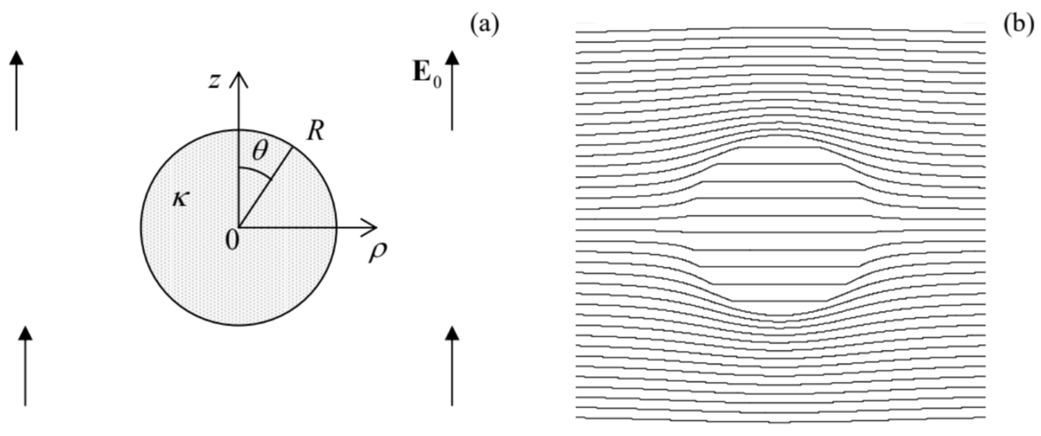
Fig. 11b shows the equipotential surfaces given by this solution, for a particular value of the dielectric constant \(\ \kappa\). Note that according to Eq. (62), at \(\ r \geq R\) the dielectric sphere, just as the conducting sphere in a similar problem, produces (on the top of the uniform external field) a pure dipole field, with the dipole moment

\[\ \mathbf{p}=4 \pi R^{3} \frac{\kappa-1}{\kappa+2} \varepsilon_{0} \mathbf{E}_{0} \equiv 3 V \frac{\kappa-1}{\kappa+2} \varepsilon_{0} \mathbf{E}_{0}, \quad \text { where } V=\frac{4 \pi}{3} R^{3}.\tag{3.64}\]

This is an evident generalization of Eq. (11), to which Eq. (64) tends at \(\ \kappa \rightarrow \infty\). By the way, this property is common: for their electrostatic (but not transport!) properties, conductors may be adequately described as dielectrics with \(\ \kappa \rightarrow \infty\).

Another remarkable feature of Eqs. (63) is that the electric field and polarization inside the sphere are uniform, with R-independent values

\[\ \mathbf{E}=\frac{3}{\kappa+2} \mathbf{E}_{0}, \quad \mathbf{D} \equiv \kappa \varepsilon_{0} \mathbf{E}=\varepsilon_{0} \frac{3 \kappa}{\kappa+2} \mathbf{E}_{0}, \quad \mathbf{P} \equiv \mathbf{D}-\varepsilon_{0} \mathbf{E}=3 \varepsilon_{0} \frac{\kappa-1}{\kappa+2} \mathbf{E}_{0} .\tag{3.65}\]

In the limit \(\ \kappa \rightarrow 1\) (the “sphere made of free space”, i.e. no sphere at all), the electric field inside it naturally tends to the external one, and its polarization disappears. In the opposite limit \(\ \kappa \rightarrow \infty\), the electric field inside the sphere vanishes. Curiously enough, in this limit the electric displacement inside the sphere remains finite: \(\ \mathbf{D} \rightarrow 3 \varepsilon_{0} \mathbf{E}_{0}\).

More complex problems with piecewise-uniform dielectrics also may be addressed by the methods discussed in Chapter 2, and in Sec. 6 I provide a few of them for the reader’s exercise. Let me discuss just one of such problems because it exhibits a new feature of the charge image method which was discussed in Secs 2.9 (and is the basis of the Green’s function approach – see Sec. 2.10). Consider the system shown in Fig. 12: a point charge near a dielectric half-space, which evidently parallels the system discussed in Sec. 2.9 – see Fig. 2.26.

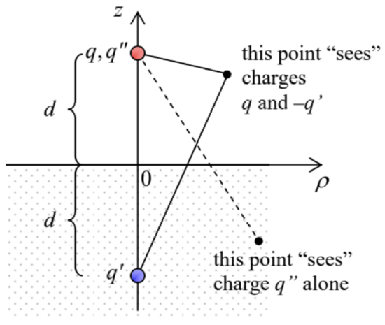Fig. 3.12. Charge images for a dielectric half-space.

As for the case of a conducting half-space, the Laplace equation for the electrostatic potential in the upper half-space \(\ z>0\) (besides the charge point \(\ \rho=0\), \(\ z=d\)) may be satisfied using a single image charge \(\ q^{\prime}\) at point \(\ \rho=0\), \(\ z=-d\), but now \(\ q^{\prime}\) may differ from \(\ (-q)\). In addition, in contrast to the case analyzed in Sec. 2.9, we should also calculate the field inside the dielectric (at \(\ z \leq 0\)). This field cannot be contributed by the image charge \(\ q^{\prime}\), because it would provide a potential divergence at its location. Thus, in that half-space we should try to use the real point source only, but maybe with a re normalized charge \(\ q^{\prime \prime}\) rather than the genuine charge \(\ q\) – see Fig. 12. As a result, we may look for the potential distribution in the form

\[\ \phi(\rho, z)=\frac{1}{4 \pi \varepsilon_{0}} \times \begin{cases}{\left[\frac{q}{\left(\rho^{2}+(z-d)^{2}\right)^{1 / 2}}+\frac{q^{\prime}}{\left(\rho^{2}+(z+d)^{2}\right)^{1 / 2}}\right],} & \text { for } z \geq 0 \\ \frac{q^{\prime \prime}}{\left(\rho^{2}+(z-d)^{2}\right)^{1 / 2}}, & \text { for } z \leq 0\end{cases}\tag{3.66}\]

at this stage with unknown \(\ q^{\prime}\) and \(\ q^{\prime\prime }\). Plugging this solution into the boundary conditions (37) and (56) at \(\ z=0\) (with \(\ \partial / \partial n=\partial / \partial z\)), we see that they are indeed satisfied (so that Eq. (66) does express the unique solution of the boundary problem), provided that the effective charges \(\ q^{\prime}\) and \(\ q^{\prime\prime}\) obey the following relations:

\[\ q-q^{\prime}=\kappa q^{\prime \prime}, \quad q+q^{\prime}=q^{\prime \prime}.\tag{3.67}\]

Solving this simple system of linear equations, we get

\[\ q^{\prime}=-\frac{\kappa-1}{\kappa+1} q, \quad q^{\prime \prime}=\frac{2}{\kappa+1} q .\tag{3.68}\]

If \(\ \kappa \rightarrow 1\), then \(\ q^{\prime} \rightarrow 0\), and \(\ q^{\prime \prime} \rightarrow q\) – both facts very natural, because in this limit (no polarization at all!) we have to recover the unperturbed field of the initial point charge in both semi-spaces. In the opposite limit \(\ \kappa \rightarrow \infty\) (which, according to our discussion of the last problem, should correspond to a conducting half-space), \(\ q^{\prime} \rightarrow-q\) (repeating the result we have discussed in detail in Sec. 2.9) and \(\ q^{\prime \prime} \rightarrow 0\). The last result means that in this limit, the electric field \(\ \mathbf{E}\) in the dielectric tends to zero – as it should.