5.7: Exercise Problems

Last updated
Save as PDF

Page ID: 57001

\( \newcommand{\vecs}[1]{\overset { \scriptstyle \rightharpoonup} {\mathbf{#1}} } \) \( \newcommand{\vecd}[1]{\overset{-\!-\!\rightharpoonup}{\vphantom{a}\smash {#1}}} \)\(\newcommand{\id}{\mathrm{id}}\) \( \newcommand{\Span}{\mathrm{span}}\) \( \newcommand{\kernel}{\mathrm{null}\,}\) \( \newcommand{\range}{\mathrm{range}\,}\) \( \newcommand{\RealPart}{\mathrm{Re}}\) \( \newcommand{\ImaginaryPart}{\mathrm{Im}}\) \( \newcommand{\Argument}{\mathrm{Arg}}\) \( \newcommand{\norm}[1]{\| #1 \|}\) \( \newcommand{\inner}[2]{\langle #1, #2 \rangle}\) \( \newcommand{\Span}{\mathrm{span}}\) \(\newcommand{\id}{\mathrm{id}}\) \( \newcommand{\Span}{\mathrm{span}}\) \( \newcommand{\kernel}{\mathrm{null}\,}\) \( \newcommand{\range}{\mathrm{range}\,}\) \( \newcommand{\RealPart}{\mathrm{Re}}\) \( \newcommand{\ImaginaryPart}{\mathrm{Im}}\) \( \newcommand{\Argument}{\mathrm{Arg}}\) \( \newcommand{\norm}[1]{\| #1 \|}\) \( \newcommand{\inner}[2]{\langle #1, #2 \rangle}\) \( \newcommand{\Span}{\mathrm{span}}\)\(\newcommand{\AA}{\unicode[.8,0]{x212B}}\)

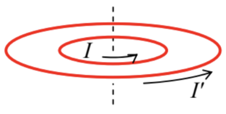
5.1. A circular wire loop, carrying a fixed dc current, has been placed inside a similar but larger loop, carrying a fixed current in the same direction – see the figure on the right. Use semi-quantitative arguments to analyze the mechanical stability of the coaxial, coplanar position of the inner loop with respect to its possible angular, axial, and lateral displacements relative to the outer loop.

Screen Shot 2022-02-09 at 1.25.06 AM.png

5.2. Two straight, plane, parallel, long, thin conducting strips of width \(\ w\), separated by distance \(\ d\), carry equal but oppositely directed currents \(\ I\) – see the figure on the right. Calculate the magnetic field in the plane located in the middle between the strips, assuming that the flowing currents are uniformly distributed across the strip widths.

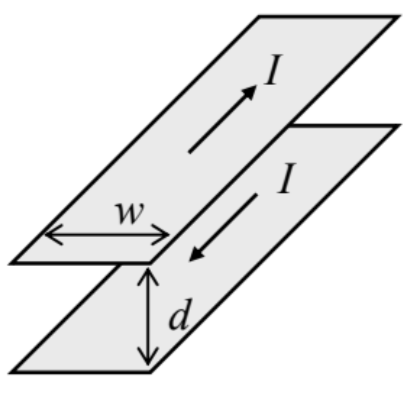
Screen Shot 2022-02-09 at 1.26.53 AM.png

5.3. For the system studied in the previous problem, but now only in the limit \(\ d << w\), calculate:

(i) the distribution of the magnetic field in space,

(ii) the vector potential of the field,

(iii) the magnetic force (per unit length) exerted on each strip, and

(iv) the magnetic energy and self-inductance of the loop formed by the strips (per unit length).

5.4. Calculate the magnetic field distribution near the center of the system of two similar, plane, round, coaxial wire coils, carrying equal but oppositely directed currents – see the figure on the right.

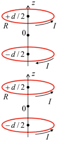
Screen Shot 2022-02-09 at 1.33.02 AM.png

5.5. The two-coil-system considered in the previous problem, now carries equal and similarly directed currents – see the figure on the right.⁶⁵ Calculate what should be the ratio \(\ d / R\) for the second derivative \(\ \partial^{2} B_{z} / \partial z^{2}\) at \(\ z = 0\) to vanish.

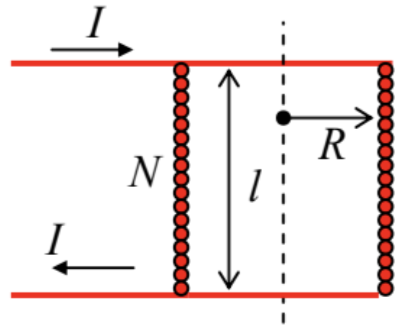
5.6. Calculate the magnetic field’s distribution along the axis of a straight solenoid (see Fig. 6a, partly reproduced on the right) with a finite length \(\ l\), and round cross-section of radius \(\ R\). Assume that the solenoid has many \(\ (N >>1, l / R)\) wire turns, uniformly distributed along its length.

Screen Shot 2022-02-09 at 1.35.22 AM.png

5.7. A thin round disk of radius \(\ R\), carrying electric charge of a constant areal density \(\ \sigma\), is being rotated around its axis with a constant angular velocity \(\ \Omega\). Calculate:

(i) the induced magnetic field on the disk’s axis,

(ii) the magnetic moment of the disk, and relate these results.

5.8. A thin spherical shell of radius \(\ R\), with charge \(\ Q\) uniformly distributed over its surface, rotates about its axis with angular velocity \(\ \omega\). Calculate the distribution of the magnetic field everywhere in space.

5.9. A sphere of radius \(\ R\), made of an insulating material with a uniform electric charge density \(\ \rho\), rotates about its diameter with angular velocity \(\ \omega\). Calculate the magnetic field distribution inside the sphere and outside it.

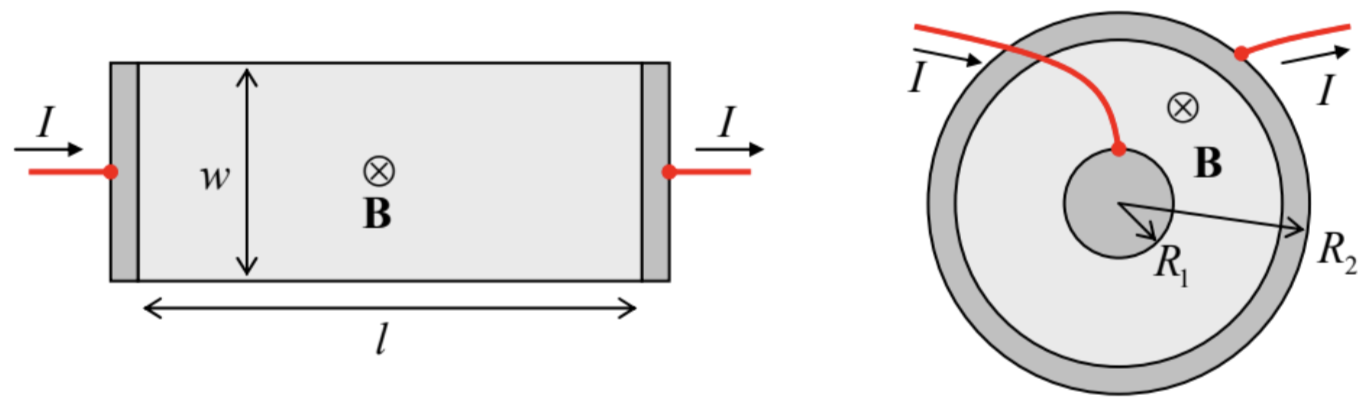
5.10. The reader is (hopefully :-) familiar with the classical Hall effect when it takes place in the usual rectangular Hall bar geometry – see the left panel of the figure below. However, the effect takes a different form in the so-called Corbino disk – see the right panel of the figure below. (Dark shading shows electrodes, with no appreciable resistance.) Analyze the effect in both geometries, assuming that in both cases the conductors are thin, planar, have a constant Ohmic conductivity \(\ \sigma\) and charge carrier density \(\ n\), and that the applied magnetic field \(\ \mathbf{B}\) is uniform and normal to conductors’ planes.

Screen Shot 2022-02-09 at 1.40.35 AM.png

5.11.* The simplest model of the famous homopolar motor⁶⁶ is a thin, round conducting disk, placed into a uniform magnetic field normal to its plane, and fed by a dc current flowing from the disk’s center to a sliding electrode (“brush”) on its rim – see the figure on the right.

(i) Express the torque rotating the disk, via its radius \(\ R\), the magnetic field \(\ \mathbf{B}\), and the current \(\ I\).

(ii) If the disk is allowed to rotate about its axis, and the motor is driven by a battery with e.m.f. \(\ \mathscr{V}\), calculate its stationary angular velocity \(\ \omega\), neglecting friction and the electric circuit’s resistance.

(iii) Now assuming that the current circuit (battery + wires + contacts + disk itself) has a non-zero resistance \(\ \mathscr{R}\), derive and solve the equation for the time evolution of \(\ \omega\), and analyze the solution.

5.12. Current \(\ I\) flows in a thin wire bent into a plane round loop of radius \(\ R\). Calculate the net magnetic flux through the plane in which the loop is located.

5.13. Prove that:

(i) the self-inductance \(\ L\) of a current loop cannot be negative, and

(ii) any inductance coefficient \(\ L_{k k’}\), defined by Eq. (60), cannot be larger than \(\ \left(L_{k k} L_{k^{\prime} k^{\prime}}\right)^{1 / 2}\).

5.14.^* Estimate the values of magnetic susceptibility due to

(i) orbital diamagnetism, and

(ii) spin paramagnetism, for a medium with negligible interaction between the induced molecular dipoles. Compare the results.

Hints: For Task (i), you may use the classical model described by Eq. (114) – see Fig. 13. For Task (ii), assume the mechanism of ordering of spontaneous magnetic dipoles \(\ \mathbf{m}_{0}\), with a magnitude \(\ m_{0}\) of the order of the Bohr magneton \(\ \mu_{\mathrm{B}}\), similar to the one sketched for electric dipoles in Fig. 3.7a.

5.15.^*Use the classical picture of the orbital (“Larmor”) diamagnetism, discussed in Sec. 5, to calculate its (small) contribution \(\ \Delta \mathbf{B}(0)\) to the magnetic field \(\ \mathbf{B}\) felt by an atomic nucleus, modeling the electrons of the atom by a spherically-symmetric cloud with an electric charge density \(\ \rho(r)\). Express the result via the value \(\ \phi(0)\) of the electrostatic potential of electrons’ cloud, and use this expression for a crude numerical estimate of the ratio \(\ \Delta B(0) / B\) for the hydrogen atom.

5.16. Calculate the (self-) inductance of a toroidal solenoid (see Fig. 6b) with the round cross-section of radius \(\ r \sim R\) (see the figure on the right), with many \(\ (N >>1, R / r)\) wire turns uniformly distributed along the perimeter, and filled with a linear magnetic material of a magnetic permeability \(\ \mu\). Check your results by analyzing the limit \(\ r<<R\).

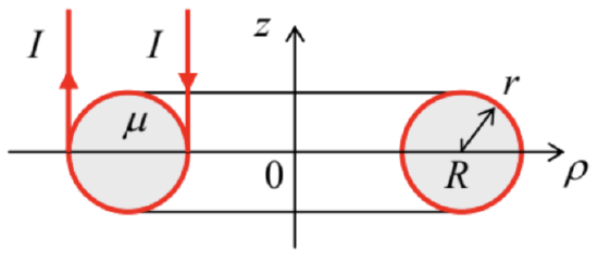
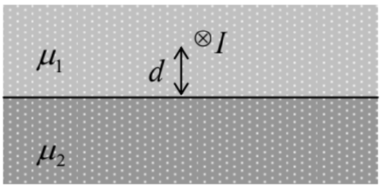
Screen Shot 2022-02-09 at 1.57.34 AM.png

5.17. A long straight, thin wire, carrying current \(\ I\), passes parallel to the plane boundary between two uniform, linear magnetics – see the figure on the right. Calculate the magnetic field everywhere in the system, and the force (per unit length) exerted on the wire.

Screen Shot 2022-02-09 at 1.58.20 AM.png

5.18. Solve the magnetic shielding problem similar to that discussed in Sec. 5.6 of the lecture notes, but for a spherical rather than cylindrical shell, with the same central cross section as shown in Fig. 16. Compare the efficiency of those two shields, for the same shell’s permeability \(\ \mu\), and the same \(\ b / a\) ratio.

5.19. Calculate the magnetic field distribution around a spherical permanent magnet with a uniform magnetization \(\ \mathbf{M}_{0}=\text { const }\).

5.20. A limited volume \(\ V\) is filled with a magnetic material with a fixed (field-independent) magnetization \(\ \mathbf{M}(\mathbf{r})\). Write explicit expressions for the magnetic field induced by the magnetization, and its potential, and recast these expressions into the forms more convenient when \(\ \mathbf{M}(\mathbf{r})=\mathbf{M}_{0}=\text { const }\) inside the volume \(\ V\).

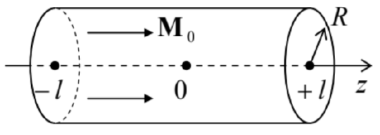
5.21. Use the results of the previous problem to calculate the distribution of the magnetic field \(\ \mathbf{H}\) along the axis of a straight permanent magnet of length \(\ 2 l\), with a round cross-section of radius \(\ R\), and a uniform magnetization \(\ \mathbf{M}_{0}\) parallel to the axis – see the figure on the right.

Screen Shot 2022-02-09 at 2.03.21 AM.png

5.22. A very broad film of thickness \(\ 2t\) is permanently magnetized normally to its plane, with a periodic checkerboard pattern, with the square of area \(\ a \times a\):

\[\ \left.\mathbf{M}\right|_{|z|<t}=\mathbf{n}_{z} M(x, y), \quad \text { with } M(x, y)=M_{0} \times \operatorname{sgn}\left(\cos \frac{\pi x}{a} \cos \frac{\pi y}{a}\right).\]

Calculate the magnetic field’s distribution in space.⁶⁷

5.23.^* Based on the discussion of the quadrupole electrostatic lens in Sec. 2.4, suggest the permanent-magnet systems that may similarly focus particles moving close to the system’s axis, and carrying:

(i) an electric charge,

(ii) no net electric charge, but a spontaneous magnetic dipole moment \(\ \mathbf{m}\).

Reference

⁶⁶ It was invented by Michael Faraday in 1821, i.e. well before his celebrated work on electromagnetic induction. The adjective “homopolar” refers to the constant “polarity” (sign) of the current; the alternative term is “unipolar”.

⁶⁷ This problem is of evident relevance for the perpendicular magnetic recording (PMR) technology, which presently dominates the high-density digital magnetic recording.