8.3: Wave Scattering

The Larmor formula may be used as the basis of the theory of scattering – the phenomenon illustrated by Fig. 4. Generally, scattering is a complex problem. However, in many cases it allows the so-called Born approximation,¹⁴ in which scattered wave field’s effect on the scattering object is assumed to be much weaker than that of the incident wave, and is neglected.

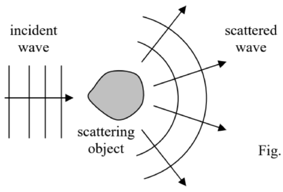Fig. 8.4. Scattering (schematically).

As the first example of this approach, let us consider the scattering of a plane wave, propagating in free space $\ \left(Z=Z_{0}, \nu=c\right)$, by a free¹⁵ charged particle whose motion may be described by non-relativistic classical mechanics. (This requires, in particular, the incident wave to be not too powerful, so that the speed of the induced charge motion remains much lower than the speed of light.) As was already discussed at the derivation of Eq. (7.32), in this case, the magnetic component of the Lorentz force (5.10) is negligible in comparison with the force $\ \mathbf{F}_{\mathrm{e}}=q \mathbf{E}$ exerted by its electric field. Thus, assuming that the incident wave is linearly polarized along some axis $\ x$, the equation of particle’s motion in the Born approximation is just $\ m \ddot{x}=q E(t)$, so that for the x-component $\ p_{x}=q x$ of its dipole moment we can write

$$\ \ddot{p}=q \ddot{x}=\frac{q^{2}}{m} E(t).\tag{8.36}$$

As we already know from Sec. 2, oscillations of the dipole moment lead to radiation of a wave with a wide angular distribution of intensity; in our case, this is the scattered wave – see Fig. 4. Its full power may be found by plugging Eq. (36) into Eq. (27):

$$\ \mathscr{P}=\frac{Z_{0}}{6 \pi c^{2}} \ddot{p}^{2}=\frac{Z_{0} q^{4}}{6 \pi c^{2} m^{2}} E^{2}(t),\tag{8.37}$$

so that for the average power we get

$$\ \overline{\mathscr{P}}=\frac{Z_{0} q^{4}}{12 \pi c^{2} m^{2}}\left|E_{\omega}\right|^{2}.\tag{8.38}$$

Since this power is proportional to the incident wave’s intensity S, it is customary to characterize the scattering ability of an object by the ratio,

$$\ \text{Full cross-section: definition}\quad\quad\quad\quad \sigma \equiv \frac{\overline{\mathscr{P}}}{\overline{S_{\text {incident }}}} \equiv \frac{\overline{\mathscr{P}}}{\left|E_{\omega}\right|^{2} / 2 Z_{0}},\tag{8.39}$$

which has the dimensionality of area, and is called the total cross-section of scattering.¹⁶ For this measure, Eq. (38) yields the famous result

$$\ \sigma=\frac{Z_{0}^{2} q^{4}}{6 \pi c^{2} m^{2}}=\frac{\mu_{0}^{2} q^{4}}{6 \pi m^{2}},\tag{8.40}$$

which is called the Thomson scattering formula,¹⁷ especially when applied to an electron. This relation is most frequently represented in the form¹⁸

$$\ \sigma=\frac{8 \pi}{3} r_{\mathrm{c}}^{2}, \quad \text { with } r_{\mathrm{c}} \equiv \frac{q^{2}}{4 \pi \varepsilon_{0}} \cdot \frac{1}{m c^{2}}.\quad\quad\quad\quad\text{Thomson scattering}\tag{8.41}$$

This constant $\ r_{\mathrm{c}}$ is called the classical radius of the particle (or sometimes the “Thomson scattering length”); for the electron $\ \left(q=-e, m=m_{\mathrm{e}}\right)$ it is close to $\ 2.82 \times 10^{-15} \mathrm{~m}$. Its possible interpretation is evident from Eq. (41) for $\ r_{\mathrm{c}}$: at that distance between two similar particles, the potential energy $\ q^{2} / 4 \pi \varepsilon_{0} r$ of their electrostatic interaction is equal to the particle’s rest-mass energy $\ m c^{2}$.¹⁹

Now we have to go back and establish the conditions at which the Born approximation, when the field of the scattered wave is negligible, is indeed valid for a point-object scattering. Since the scattered wave’s intensity, described by Eq. (26), diverges as $\ 1 / r^{2}$, according to the definition (39) of the cross-section, it may become comparable to $\ S_{\text {incident }}$ at $\ r^{2} \sim \sigma$. However, Eq. (38) itself is only valid if $\ r >> \lambda$, so that the Born approximation does not lead to a contradiction only if

$$\ \sigma<<\lambda^{2}.\tag{8.42}$$

For the Thompson scattering by an electron, this condition means $\ \lambda >> r_{\mathrm{c}} \sim 3 \times 10^{-15} \mathrm{~m}$ and is fulfilled for all frequencies up to very hard $\ \gamma$-rays with photon energies ~ 100 MeV.

Possibly the most notable feature of the result (40) is its independence of the wave frequency. As it follows from its derivation, particularly from Eq. (37), this independence is intimately related to the unbound character of charge motion. For bound charges, say for electrons in gas molecules, this result is only valid if the wave frequency $\ \omega$ is much higher than the eigenfrequencies $\ \omega_{j}$ of most important quantum transitions. In the opposite limit, $\ \omega<<\omega_{j}$, the result is dramatically different. Indeed, in this limit we may approximate the molecule’s dipole moment by its static value (3.48):

$$\ \mathbf{p}=\alpha \mathbf{E}.\tag{8.43}$$

In the Born approximation, and in the absence of the molecular field effects mentioned in Sec. 3.3, E in this expression is just the incident wave’s field, and we can use Eq. (28) to calculate the power of the wave scattered by a single molecule:

$$\ \overline{\mathscr{P}}=\frac{Z_{0} \omega^{4}}{4 \pi c^{2}} \alpha^{2}\left|E_{\omega}\right|^{2}.\tag{8.44}$$

Now, using the last form of the definition (39) of the cross-section, we get a very simple result,

$$\ \sigma=\frac{Z_{0}^{2} \omega^{4}}{6 \pi c^{2}} \alpha^{2},\tag{8.45}$$

showing that in contrast to Eq. (40), at low frequencies $\ \sigma$ changes as fast as $\ \omega^{4}$.

Now let us explore the effect of such Rayleigh scattering on wave propagation in a gas, with a relatively low volumic density $\ n$. We may expect (and will prove in the next section) that due to the randomness of molecule positions, the waves scattered by individual molecules may be treated as incoherent ones, so that the total scattering power may be calculated just as the sum of those scattered by each molecule. We can use this fact to write the balance of the incident’s wave intensity in a small volume $\ dV$ of length (along the incident wave direction) $\ dz$, and area $\ A$ across it. Since such a segment includes $\ n d V=n A d z$ molecules, and according to Eq. (39), each of them scatters power $\ S \sigma=\mathscr{P} \sigma / A$, the total scattered power is $\ n \mathscr{P} \sigma d z$; hence the incident power’s change is

$$\ d \mathscr{P} \equiv-n \sigma \mathscr{P} d z.\tag{8.46}$$

Comparing this equation with the definition (7.213) of the wave attenuation constant, applied to the scattering,²⁰

$$\ d \mathscr{P} \equiv-\alpha_{\text {scat }} \mathscr{P} d z.\tag{8.47}$$

we see that this effect gives the following contribution to attenuation: $\ \alpha_{\text {scat }}=n \sigma$. From here, using Eq. (3.50) to write $\ \alpha=\varepsilon_{0}(\kappa-1) / n$, where $\ \kappa$ is the dielectric constant, and Eq. (45) for $\ \sigma$, we get

$$\ \text{Rayleigh scattering}\quad\quad\quad\quad \alpha_{\text {scat }}=\frac{k^{4}}{6 \pi n}(\kappa-1)^{2}, \quad \text { where } k \equiv \frac{2 \pi}{\lambda_{0}}=\frac{\omega}{c}.\tag{8.48}$$

This is the famous Rayleigh scattering formula, which in particular explains the colors of blue sky and red sunsets. Indeed, through the visible light spectrum, $\ \omega$ changes almost two-fold; as a result, the scattering of blue components of sunlight is an order of magnitude higher than that of its red components. For the air near the Earth’s surface, $\ \kappa-1 \approx 6 \times 10^{-4}$, and $\ n \sim 2.5 \times 10^{25} \mathrm{~m}^{-3}$ – see Sec. 3.3. Plugging these numbers into Eq. (48), we see that the effective length $\ l_{\text {scat }} \equiv 1 / \alpha_{\text {scat }}$ of scattering is ~30 km for the blue light and ~200 km for the red light.²¹ The effective thickness $\ h$ of the Earth’s atmosphere is ~10 km, so that the Sun looks just a bit yellowish during most of the day. However, an elementary geometry shows that on the sunset, the light should pass the length $\ l \sim\left(R_{\mathrm{E}} h\right)^{1 / 2} \approx 300 \mathrm{~km}$ to reach an Earth-surface observer; as a result, the blue components of the Sun’s light spectrum are almost completely scattered out, and even the red components are weakened substantially.

---

Reference

¹⁴ Named after Max Born, one of the founding fathers of quantum mechanics. However, the basic idea of this approach to EM waves was developed much earlier (in 1881) by Lord Rayleigh – born John William Strutt.

¹⁵ As Eq. (7.30) shows, this calculation is also valid for an oscillator with a low own frequency, $\ \omega_{0}<<\omega$.

¹⁶ This definition parallels those accepted in the classical and quantum theories of particle scattering - see, e.g., respectively, CM Sec. 3.5 and QM Sec. 3.3.

¹⁷ Named after Sir Joseph John (“JJ”) Thomson, the discoverer of the electron – and isotopes as well! He should not be confused with his son, G. P. Thomson, who discovered (simultaneously with C. Davisson and L. Germer) quantum-mechanical wave properties of the same electron.

¹⁸ In the Gaussian units, this formula looks like $\ r_{\mathrm{c}}=q^{2} / m c^{2}$ (giving, of course, the same numerical values: for the electron, $\ r_{\mathrm{c}} \approx 2.82 \times 10^{-13} \mathrm{~cm}$). This classical quantity should not be confused with the particle’s Compton wavelength $\ \lambda_{\mathrm{C}} \equiv 2 \pi \hbar / m \mathrm{c}$ (for the electron, close to $\ 2.24 \times 10^{-12} \mathrm{~m}$), which naturally arises in quantum electrodynamics – see a brief discussion in the next chapter, and also QM Sec. 1.1.

¹⁹ It is fascinating how smartly has the relativistic expression $\ m c^{2}$ sneaked into the result (40)-(41), which was obtained using the non-relativistic equation (36) of the particle motion. This was possible because the calculation engaged electromagnetic waves, which propagate with the speed of light, and whose quanta (photons), as a result, may be frequently treated as relativistic (moreover, ultra-relativistic) particles – see the next chapter.

²⁰ I am sorry for using the same letter $\ (\alpha)$ for both the molecular polarizability and the wave attenuation, but both notations are traditional. Hopefully, the subscript “scat”, marking $\ \alpha$ in the latter meaning, minimizes the possibility of confusion.

²¹ These values are approximate because both $\ n$ and $\ (\kappa-1)$ vary through the atmosphere’s thickness.