
8.4: Interference and Diffraction


- Last updated
- Mar 5, 2022
- Save as PDF

( \newcommand{\kernel}{\mathrm{null}\,}\)
Now let us discuss scattering by objects with a size of the order of, or even larger than \ \lambda. For such extended objects, the phase difference factors (neglected above) step in, leading in particular to the important effects of interference and diffraction. These effects show up not as much in the total power of the scattered radiation, as in its angular distribution. It is traditional to characterize this distribution by the differential cross-section defined as
\ \frac{d \sigma}{d \Omega} \equiv \frac{\bar{S}_{r} r^{2}}{\overline{S_{\text {incident }}}},\quad\quad\quad\quad \text{Differential cross-section}\tag{8.49}
where \ r is the distance from the scatterer, at which the scattered wave is observed.22 Both the definition and the notation may become more clear if we notice that according to Eq. (26), at large distances \ (r >>a), the numerator of the right-hand side of Eq. (49), and hence the differential cross-section as a whole, do not depend on \ r, and that its integral over the total solid angle \ \Omega=4 \pi coincides with the total cross-section defined by Eq. (39):
\ \oint_{4 \pi} \frac{d \sigma}{d \Omega} d \Omega=\frac{1}{\overline{S_{\text {incident }}}} r^{2} \oint_{4 \pi} \bar{S}_{r} d \Omega=\frac{1}{\overline{S_{\text {incident }}}} \oint_{r=\text { const }} \overline{S_{r}} d^{2} r=\frac{\overline{\mathscr{P}}}{\overline{S_{\text {incident }}}} \equiv \sigma.\tag{8.50}
For example, according to Eq. (26), the angular distribution of the radiation scattered by a single dipole is rather broad; in particular, in the quasistatic case (43), and in the Born approximation,
\ \frac{d \sigma}{d \Omega}=\left(\frac{\alpha k^{2}}{4 \pi \varepsilon_{0}}\right)^{2} \sin ^{2} \Theta.\tag{8.51}
If the wave is scattered by a small dielectric body, with a characteristic size \ a<<\lambda (i.e., \ k a<<1), then all its parts re-radiate the incident wave coherently. Hence, we can calculate it similarly, just replacing the molecular dipole moment (43) with the total dipole moment of the object – see Eq. (3.45):
\ \mathbf{p}=\mathbf{P} V=(\kappa-1) \varepsilon_{0} \mathbf{E} V,\tag{8.52}
where \ V \sim a^{3} is the body’s volume. As a result, the differential cross-section may be obtained from Eq. (51) with the replacement \ \alpha_{\mathrm{mol}} \rightarrow(\kappa-1) \varepsilon_{0} V:
\ \frac{d \sigma}{d \Omega}=\left(\frac{k^{2} V}{4 \pi}\right)^{2}(\kappa-1)^{2} \sin ^{2} \Theta,\tag{8.53}
i.e. follows the same \ \sin ^{2} \Theta law.
The situation for extended objects, with at least one dimension of the order of (or larger than) the wavelength, is different: here we have to take into account the phase shifts between the re-radiation by various parts of the body. Let us analyze this issue first for an arbitrary collection of similar point scatterers located at points \ \mathbf{r}_{j}. If the wave vector of the incident plane wave is \ \mathbf{k}_{0}, the wave’s field has the phase factor \ \exp \left\{i \mathbf{k}_{0} \cdot \mathbf{r}\right\} – see Eq. (7.79). At the location \ \mathbf{r}_{j} of the \ j^{\text {th }} scattering center, this factor equals to \ \exp \left\{i \mathbf{k}_{0} \cdot \mathbf{r}_{j}\right\}, so that the local dipole vectors p, and the scattered wave they create, are proportional to this factor. On its way to the observation point r, the scattered wave, with the wave
vector k (with \ k=k_{0}), acquires an additional phase factor \ \exp \left\{\mathbf{i k} \cdot\left(\mathbf{r}-\mathbf{r}_{j}\right)\right\}, so that the scattered wave
field is proportional to
\ \exp \left\{i \mathbf{k}_{0} \cdot \mathbf{r}_{j}+i \mathbf{k}\left(\mathbf{r}-\mathbf{r}_{j}\right)\right\} \equiv e^{i \mathbf{k} \cdot \mathbf{r}} \exp \left\{-i\left(\mathbf{k}-\mathbf{k}_{0}\right) \cdot \mathbf{r}_{j}\right\}.\tag{8.54}
Since the first factor in the last expression does not depend on \ \mathbf{r}_{j}, to calculate the total scattering wave, it is sufficient to sum up the last phase factors, \ \exp \left\{-\mathbf{i} \mathbf{q} \cdot \mathbf{r}_{j}\right\}, where the vector
\ \mathbf{q} \equiv \mathbf{k}-\mathbf{k}_{0}\tag{8.55}
has the physical sense of the wave vector change at scattering.23 It may look like the phase factor depends on the choice of the reference frame. However, according to Eq. (7.42), the average intensity of the scattered wave is proportional to \ E_{\omega} E_{\omega}{ }^{*}, i.e. to the following real scalar function of the vector q:
\ \text{Scattering function}\quad\quad\quad\quad F(\mathbf{q})=\left(\sum_{j} \exp \left\{-i \mathbf{q} \cdot \mathbf{r}_{j}\right\}\right)\left(\sum_{j^{\prime}} \exp \left\{-i \mathbf{q} \cdot \mathbf{r}_{j^{\prime}}\right\}\right)^{*}=\sum_{j, j^{\prime}} \exp \left\{i \mathbf{q} \cdot\left(\mathbf{r}_{j}-\mathbf{r}_{j^{\prime}}\right)\right\} \equiv|I(\mathbf{q})|^{2},\tag{8.56}
where the complex function
\ \text{Phase sum}\quad\quad\quad\quad I(\mathbf{q}) \equiv \sum_{j} \exp \left\{-i \mathbf{q} \cdot \mathbf{r}_{j}\right\}\tag{8.57}
is called the phase sum, and may be calculated in any reference frame, without affecting the final result given by Eq. (56).
So, besides the \ \sin ^{2} \Theta factor, the differential cross-section (49) of scattering by an extended object is also proportional to the scattering function (56). Its double-sum form is convenient to notice that for a system of many \ (N >> 1) of similar but randomly located scatterers, only the terms with \ j=j^{\prime} accumulate at summation, so that \ F(\mathbf{q}), and hence \ d \sigma / d \Omega, scale as \ N, rather than \ N^{2} – thus justifying again our treatment of the Rayleigh scattering problem in the previous section.
Let us start using Eq. (56) by applying it to a simple problem of just two similar small scatterers, separated by a fixed distance \ a:
\ F(\mathbf{q})=\sum_{j, j^{\prime}=1}^{2} \exp \left\{i \mathbf{q} \cdot\left(\mathbf{r}_{j}-\mathbf{r}_{j^{\prime}}\right)\right\}=2+\exp \left\{-i q_{a} a\right\}+\exp \left\{i q_{a} a\right\}=2\left(1+\cos q_{a} a\right)=4 \cos ^{2} \frac{q_{a} a}{2},\tag{8.58}
where \ q_{a} \equiv \mathbf{q} \cdot \mathbf{a} / a is the component of the vector q along the vector a connecting the scatterers. The apparent simplicity of this result may be a bit misleading, because the mutual plane of the vectors k and \ \mathbf{k}_{0} (and hence of the vector q) does not necessarily coincide with the mutual plane of the vectors \ \mathbf{k}_{0} and \ \mathbf{E}_{\omega}, so that the scattering angle \ \theta between k and \ \mathbf{k}_{0} is generally different from \ (\pi / 2-\Theta) – see Fig. 5. Moreover, the angle between the vectors q and a (within their common plane) is one more parameter independent of both \ \theta and \ \Theta. As a result, the angular dependence of the scattered wave’s intensity (and hence \ d \sigma /d \Omega), which depends on all three angles, may be rather involved, but some of its details do not affect the basic physics of the interference/diffraction.
 Fig. 8.5. The angles important for the general scattering problem.
This is why let me consider in detail only the simple cases when the vectors \ \mathbf{k}, \ \mathbf{k}_{0}, and a all lie in the same plane, with \ \mathbf{k}_{0} normal to a – see Figs. 6.
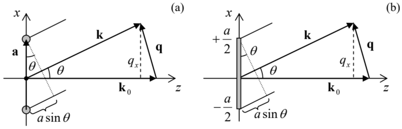 Fig. 8.6. The simplest cases of (a) interference and (b) diffraction.
For the two-point scatterer shown in Fig. 6a, with our choice of coordinates, \ q_{a}=q_{x}=k \sin \theta, and Eq. (58) is reduced to
\ F(\mathbf{q})=4 \cos ^{2} \frac{k a \sin \theta}{2}.\tag{8.59}
This function always has two maxima, at \ \theta=0 and \ \theta=\pi, and, if the product \ ka is large enough, other maxima24 at the special angles \ \theta_{n} that satisfy the simple condition
\ k a \sin \theta_{n}=2 \pi n, \quad \text { i.e. } a \sin \theta_{n}=n \lambda.\quad\quad\quad\quad \text{Bragg condition} \tag{8.60}
As Fig. 6a shows, this condition may be readily understood as that of the in-phase addition (the constructive interference) of two coherent waves scattered from the two points, when the difference between their paths toward the observer, \ a \sin \theta, equals to an integer number of wavelengths. At each such maximum, \ F=4, due to the doubling of the wave amplitude and hence quadrupling its power.
If the distance between the point scatterers is large \ (k a >>1), the first maxima (60) correspond to small scattering angles, \ \theta<<1. For this region, Eq. (59) is reduced to a simple periodic dependence of function \ F on the angle \ \theta. Moreover, within the range of small \ \theta, the wave polarization factor \ \sin ^{2} \Theta is virtually constant, so that the scattered wave intensity, and hence the differential cross-section are also very simple:
\ \frac{d \sigma}{d \Omega} \propto F(\mathbf{q})=4 \cos ^{2} \frac{k a \theta}{2}.\quad\quad\quad\quad \text{Young’s interference pattern}\tag{8.61}
This simple interference pattern is well known from Young’s two-slit experiment.25 (As will be discussed in the next section, the theoretical description of the two-slit experiment is more complex than that of the Born scattering, but is preferable experimentally, because at such scattering, the wave of intensity (61) has to be observed on the backdrop of a much stronger incident wave that propagates in almost the same direction, \ \theta=0.)
A very similar analysis of scattering from \ N > 2 similar, equidistant scatterers, located along the same straight line shows that the positions (60) of the constructive interference maxima do not change (because the derivation of this condition is still applicable to each pair of adjacent scatterers), but the increase of \ N makes these peaks sharper and sharper. Leaving the quantitative analysis of this system for the reader’s exercise, let me jump immediately to the limit \ N \rightarrow 0, in which we may ignore the scatterers’ discreteness. The resulting pattern is similar to that at scattering by a continuous thin rod (see Fig. 6b), so let us first spell out the Born scattering formula for an arbitrary an extended, continuous, uniform dielectric body. Transferring Eq. (56) from the sum to an integral, for the differential cross-section we get
\ \frac{d \sigma}{d \Omega}=\left(\frac{k^{2}}{4 \pi}\right)^{2}(\kappa-1)^{2} F(\mathbf{q}) \sin ^{2} \Theta \equiv\left(\frac{k^{2}}{4 \pi}\right)^{2}(\kappa-1)^{2}|I(\mathbf{q})|^{2} \sin ^{2} \Theta,\tag{8.62}
where \ I(\mathbf{q}) now becomes the phase integral,26
\ \text{Phase integral}\quad\quad\quad\quad I(\mathbf{q})=\int_{V} \exp \left\{-i \mathbf{q} \cdot \mathbf{r}^{\prime}\right\} d^{3} r^{\prime},\tag{8.63}
with the dimensionality of volume.
Now we may return to the particular case of a thin rod (with both dimensions of the cross-section’s area \ A much smaller than \ \lambda, but an arbitrary length \ a), otherwise keeping the same simple geometry as for two-point scatterers – see Fig. 6b. In this case, the phase integral is just
\ \text{Fraunhofer diffraction integral}\quad I(\mathbf{q})=A \int_{-a / 2}^{+a / 2} \exp \left\{-i q_{x} x^{\prime}\right) d x^{\prime}=A \frac{\exp \left\{-i q_{x} a / 2\right\}-\exp \left\{-i q_{x} a / 2\right\}}{-i q} \equiv V \frac{\sin \xi}{\xi},\tag{8.64}
where \ V = Aa is the volume of the rod, and \ \xi is the dimensionless argument defined as
\ \xi \equiv \frac{q_{x} a}{2} \equiv \frac{k a \sin \theta}{2}.\tag{8.65}
The fraction participating in the last form of Eq. (64) is met in physics so frequently that it has deserved the special name of the sinc (not “sync”, please!) function (see Fig. 7):
\ \operatorname{sinc} \xi \equiv \frac{\sin \xi}{\xi}.\quad\quad\quad\quad\text{Sinc function}\tag{8.66}
It vanishes at all points \ \xi_{n}=\pi n, with integer \ n, besides such point with \ n=0: \ \operatorname{sinc} \xi_{0} \equiv \operatorname{sinc} 0=1.
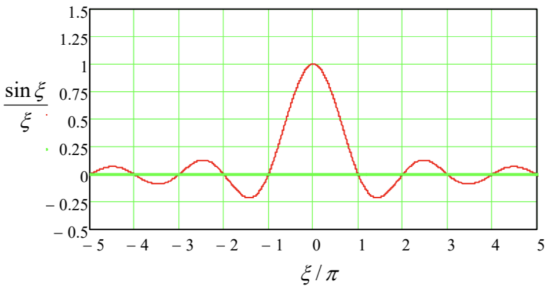 Fig. 8.7. The sinc function.
The function \ F(\mathbf{q})=V^{2} \operatorname{sinc}^{2} \xi, given by Eq. (64) and plotted with the red line in Fig. 8, is called the Fraunhofer diffraction pattern.27
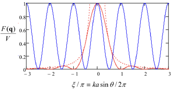
Note that it oscillates with the same argument period \ \Delta(k a \sin \theta)=2 \pi / k a as the interference pattern (61) from two-point scatterers (shown with the blue line in Fig. 8). However, at the interference, the scattered wave intensity vanishes at angles \ \theta_{n}{ }^{\prime} that satisfy the condition
\ \frac{k a \sin \theta_{n}^{\prime}}{2 \pi}=n+\frac{1}{2},\tag{8.67}
i.e. when the optical paths difference \ a \sin \alpha equals to a semi-integer number of wavelengths \ \lambda / 2=\pi / k, and hence the two waves from the scatterers reach the observer in anti-phase – the so-called destructive interference. On the other hand, for the diffraction on a continuous rod the minima occur at a different set of scattering angles:
\ \frac{k a \sin \theta_{n}}{2 \pi}=n,\tag{8.68}
i.e. exactly where the two-point interference pattern has its maxima – see Fig. 8 again. The reason for this relation is that the wave diffraction on the rod may be considered as a simultaneous interference of waves from all its elementary fragments, and exactly at the observation angles when the rod edges give waves with phases shifted by \ 2 \pi n, the interior points of the rod give waves with all possible phases, with their algebraic sum equal to zero. As even more visible in Fig. 8, at the diffraction, the intensity oscillations are limited by a rapidly decreasing envelope function \ 1 / \xi^{2} – while at the two-point interference, the oscillations retain the same amplitude. The reason for this fast decrease is that with each Fraunhofer diffraction period, a smaller and smaller fraction of the road gives an unbalanced contribution to the scattered wave.
If the rod’s length is small \ (k a<<1, \text { i.e. } a<<\lambda), then the sinc function’s argument \ \xi is small at all scattering angles \ \theta, so \ I(\mathbf{q}) \approx V, and Eq. (62) is reduced to Eq. (53). In the opposite limit, \ a >> \lambda, the first zeros of the function \ I(\mathbf{q}) correspond to very small angles \ \theta, for which \ \sin \Theta \approx 1, so that the differential cross-section is just
\ \frac{d \sigma}{d \Omega}=\left(\frac{k^{2}}{4 \pi}\right)^{2}(\kappa-1)^{2} \operatorname{sinc}^{2} \frac{k a \theta}{2},\tag{8.69}
i.e. Fig. 8 shows the scattering intensity as a function of the direction toward the observation point – if this point is within the plane containing the rod.
Finally, let us discuss a problem of large importance for applications: calculate the positions of the maxima of the interference pattern arising at the incidence of a plane wave on a very large 3D periodic system of point scatterers. For that, first of all, let us quantify the notion of 3D periodicity. The periodicity in one dimension is simple: the system we are considering (say, the positions of point scatterers) should be invariant with respect to the linear translation by some period a, and hence by any multiple sa of this period, where s is any integer. Anticipating the 3D generalization, we may require any of the possible translation vectors \ R, to that the system is invariant, to be equal \ s \mathbf{a}, where the primitive vector a is directed along the (only) axis of the 1D system.
Now we are ready for the common definition of the 3D periodicity – as the invariance of the system with respect to the translation by any vector of the following set:
\ \text{Bravais lattice}\quad\quad\quad\quad \mathbf{R}=\sum_{l=1}^{3} s_{l} \mathbf{a}_{l},\tag{8.70}
where \ s_{l} are 3 independent integers, and \ \left\{\mathbf{a}_{l}\right\} is a set of 3 linearly-independent primitive vectors. The set of geometric points described by Eq. (70) is called the Bravais lattice (first analyzed in detail, circa 1850, by Auguste Bravais). Perhaps the most nontrivial feature of this relation is that the vectors \ \mathbf{a}_{l} should not necessarily be orthogonal to each other. (That requirement would severely restrict the set of possible lattices, and make it unsuitable for the description, for example, of many solid-state crystals.) For the scattering problem we are considering, let us assume that the position \ \mathbf{r}_{j} of each scatterer
coincides with one of the points R of some Bravais lattice, with a given set of primitive vectors \ \mathbf{a}_{l}, so that the index \ j is coding the set of integers \ \left\{s_{1}, s_{2}, s_{3}\right\}.
Now let us consider a similarly defined Bravais lattice, but in the reciprocal (wave-number) space, numbered by independent integers \ \left\{t_{1}, t_{2}, t_{3}\right\}:
\ \text{Reciprocal lattice}\quad\quad\quad\quad \mathbf{Q}=\sum_{m=1}^{3} t_{m} \mathbf{b}_{m}, \quad \text { with } \mathbf{b}_{m}=2 \pi \frac{\mathbf{a}_{m^{\prime \prime}} \times \mathbf{a}_{m^{\prime}}}{\mathbf{a}_{m} \cdot\left(\mathbf{a}_{m^{\prime \prime}} \times \mathbf{a}_{m^{\prime}}\right)},\tag{8.71}
where in the last expression, the indices \ m, \ m’, and \ m^{\prime \prime} are all different. This is the so-called reciprocal lattice, which plays an important role in all physics of periodic structures, in particular in the quantum energy-band theory.28 To reveal its most important property, and thus justify the above definition of the primitive vectors \ \mathbf{b}_{m}, let us calculate the following scalar product:
\ \mathbf{R} \cdot \mathbf{Q} \equiv \sum_{l, m=1}^{3} s_{l} t_{m} \mathbf{a}_{l} \cdot \mathbf{b}_{m} \equiv 2 \pi \sum_{l, m=1}^{3} s_{l} t_{m} \mathbf{a}_{l} \cdot \frac{\mathbf{a}_{m^{\prime \prime}} \times \mathbf{a}_{m^{\prime}}}{\mathbf{a}_{m} \cdot\left(\mathbf{a}_{m^{\prime \prime}} \times \mathbf{a}_{m^{\prime}}\right)} \equiv 2 \pi \sum_{l, m=1}^{3} s_{l} t_{k} \frac{\mathbf{a}_{l} \cdot\left(\mathbf{a}_{m^{\prime \prime}} \times \mathbf{a}_{m^{\prime}}\right)}{\mathbf{a}_{m} \cdot\left(\mathbf{a}_{m^{\prime \prime}} \times \mathbf{a}_{m^{\prime}}\right)}.\tag{8.72}
Applying to the numerator of the last fraction the operand rotation rule of vector algebra,29 we see that it is equal to zero if \ l \neq m, while for \ l = m the whole fraction is evidently equal to 1. Thus the double sum (72) is reduced to a single sum:
\ \mathbf{R} \cdot \mathbf{Q}=2 \pi \sum_{l=1}^{3} s_{l} t_{l}=2 \pi \sum_{l=1}^{3} n_{l},\tag{8.73}
where each of the products \ n_{l} \equiv s_{l} t_{l} is an integer, and hence their sum,
\ n \equiv \sum_{l=1}^{3} n_{l} \equiv s_{1} t_{1}+s_{2} t_{2}+s_{3} t_{3},\tag{8.74}
is an integer as well, so that the main property of the direct/reciprocal lattice couple is very simple:
\ \mathbf{R} \cdot \mathbf{Q}=2 \pi n, \quad \text { and } \exp \{-i \mathbf{R} \cdot \mathbf{Q}\}=1.\tag{8.75}
Now returning to the scattering function (56), we see that if the vector \ \mathbf{q} \equiv \mathbf{k}-\mathbf{k}_{0} coincides with any vector Q of the reciprocal lattice, then all terms of the phase sum (57) take their largest possible values (equal to 1), and hence the sum as the whole is largest as well, giving a constructive interference maximum. This equality, \ \mathbf{q}=\mathbf{Q}, where Q is given by Eq. (71), is called the von Laue condition (named after Max von Laue) of the constructive interference; it is, in particular, the basis of all field of the X-ray crystallography of solids and polymers – the main tool for revealing their atomic/molecular structure.30
In order to recast the von Laue condition is a more vivid geometric form, let us consider one of the vectors Q of the reciprocal lattice, corresponding to a certain integer n in Eq. (75), and notice that if that relation is satisfied for one point R of the direct Bravais lattice (70), i.e. for one set of the integers \ \left\{s_{1}, s_{2}, s_{3}\right\}, it is also satisfied for a 2D system of other integer sets, which may be parameterized, for example, by two integers \ S_{1} and \ S_{2}:
\ s_{1}^{\prime}=s_{1}+S_{1} t_{3}, \quad s_{2}^{\prime}=s_{2}+S_{2} t_{3}, \quad s_{3}^{\prime}=s_{3}-S_{1} t_{1}-S_{2} t_{2}.\tag{8.76}
Indeed, each of these sets has the same value of the integer \ n, defined by Eq. (74), as the original one:
\ n^{\prime} \equiv s_{1}^{\prime} t_{1}+s_{2}^{\prime} t_{2}+s_{3}^{\prime} t_{3} \equiv\left(s_{1}+S_{1} t_{3}\right) t_{1}+\left(s_{2}+S_{2} t_{3}\right) t_{2}+\left(s_{3}-S_{1} t_{1}-S_{2} t_{2}\right) t_{3}=n.\tag{8.77}
Since according to Eq. (75), the vector of the distance between any pair of the corresponding points of the direct Bravais lattice (70),
\ \Delta \mathbf{R}=\Delta S_{1} t_{3} \mathbf{a}_{1}+\Delta S_{2} t_{3} \mathbf{a}_{2}-\left(\Delta S_{1} t_{1}+\Delta S_{2} t_{2}\right) \mathbf{a}_{3},\tag{8.78}
satisfies the condition \ \Delta \mathbf{R} \cdot \mathbf{Q}=2 \pi \Delta n=0, this vector is normal to the (fixed) vector Q. Hence, all the points corresponding to the 2D set (76), with arbitrary integers \ S_{1} and \ S_{2}, are located on one geometric plane, called the crystal (or “lattice”) plane. In a 3D system of \ N >>1 scatterers (such as \ N \sim 10^{20} atoms in a \ \sim 1-\mathrm{mm}^{3} solid crystal), with all linear dimensions comparable, such a plane contains \ \sim N^{2 / 3}>>1 points. As a result, the constructive interference peaks are very sharp.
Now rewriting Eq. (75) as a relation for the vector \ \mathbf { R's } component along the vector Q,
\ R_{Q}=\frac{2 \pi}{Q} n, \quad \text { where } R_{Q} \equiv \mathbf{R} \cdot \mathbf{n}_{Q} \equiv \mathbf{R} \cdot \frac{\mathbf{Q}}{Q}, \quad \text { and } Q \equiv|\mathbf{Q}|,\tag{8.79}
we see that the parallel crystal planes, corresponding to different numbers \ n (but the same Q) are located in space periodically, with the smallest distance
\ d=\frac{2 \pi}{Q},\tag{8.80}
so that the von Laue condition \ \mathbf{q}=\mathbf{Q} may be rewritten as the following rule for the possible magnitudes of the scattering vector \ \mathbf{q} \equiv \mathbf{k}-\mathbf{k}_{0}:
\ q=\frac{2 \pi n}{d}.\tag{8.81}
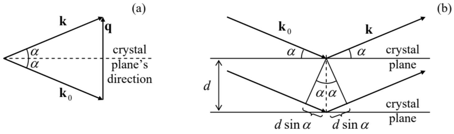
Figure 9a shows the diagram of the three wave vectors \ \mathbf{k}, \ \mathbf{k}_{0}, and \ \mathbf{q}, taking into account the elastic scattering condition \ |\mathbf{k}|=\left|\mathbf{k}_{0}\right|=k \equiv 2 \pi / \lambda. From the diagram, we immediately get the famous Bragg rule31 for the (equal) angles \ \alpha \equiv \theta / 2v between the crystal plane and each of the vectors \ \mathbf{k} and \ \mathbf{k}_{0}:
\ \text{Bragg rule}\quad\quad\quad\quad k \sin \alpha=\frac{q}{2}=\frac{\pi n}{d} \quad\quad \text{i.e. }2d \sin \alpha = n\lambda.\tag{8.82}
The physical sense of this relation is very simple – see Fig. 9b drawn in the “direct” space of the radius-vectors r, rather than in the reciprocal space of the wave vectors, as Fig. 9a. It shows that if the Bragg condition (82) is satisfied, the total difference \ 2 d \sin \alpha of the optical paths of two waves, partly reflected from the adjacent crystal planes, is equal to an integer number of wavelengths, so these waves interfere constructively.
Finally, note that the von Laue and Bragg rules, as well as the similar condition (60) for the 1D system of scatterers, are valid not only in the Born approximation but also follow from any adequate theory of scattering, because the phase sum (57) does not depend on the magnitude of the wave propagating from each elementary scatterer, provided that they are all equal.
Reference
22 Just as in the case of the total cross-section, this definition is also similar to that accepted at the particle scattering – see, e.g., CM Sec. 3.5 and QM Sec. 3.3.
23 In quantum mechanics, \ \hbar \mathbf{q} has a very clear sense of the momentum transferred from the scattering object to the scattered particle (for example, a photon), and this terminology is sometimes smuggled even into classical electrodynamics texts.
24 In optics, such intensity maxima, observed as bright spots/stripes on a screen, are called interference fringes.
25 This experiment was described in 1803 by Thomas Young – one more universal genius of science, who has also introduced the Young modulus in the elasticity theory (see, e.g., CM Chapter 7), besides numerous other achievements – including deciphering Egyptian hieroglyphs! It is fascinating that the first clear observation of wave interference was made as early as 1666 by another genius, Sir Isaac Newton, in the form of so-called Newton’s rings. Unbelievably, Newton failed to give the most natural explanation of his observations – perhaps because he was violently opposed to the very idea of light as a wave, which was promoted in his times by others, notably including Christian Huygens. Due to Newton’s enormous authority, only Young’s two-slit experiments more than a century later have firmly established the wave picture of light – to be replaced by the dualistic wave/photon picture formalized by quantum electrodynamics (see, e.g., QM Ch. 9), in one more century.
26 Since the observation point’s position r does not participate in this formula explicitly, the prime sign in r’ could be dropped, but I keep it as a reminder that the integral is taken over points r’ of the scattering object.
27 It is named after Joseph von Fraunhofer (1787-1826) – who has invented the spectroscope, developed the diffraction grating (see below), and also discovered the dark Fraunhofer lines in Sun’s spectrum.
28 See, e.g., QM Sec. 3.4, where several particular Bravais lattices R, and their reciprocals Q, are considered.
29 See, e.g., MA Eq. (7.6).
30 For more reading on this important topic, I can recommend, for example, the classical monograph by B. Cullity, Elements of X-Ray Diffraction, 2nd ed., Addison-Wesley, 1978. (Note that its title uses the alternative name of the field, once again illustrating how blurry the boundary between the interference and diffraction is.)
31 Named after Sir William Bragg and his son, Sir William Lawrence Bragg, who were first to demonstrate (in 1912) the X-ray diffraction by atoms in crystals. The Braggs’ experiments have made the existence of atoms (before that, a hypothetical notion, which had been ignored by many physicists) indisputable.