8.6: Fresnel and Fraunhofer Diffraction Patterns

Now let us use the Huygens principle to analyze a (slightly) more complex problem: plane wave’s diffraction on a long, straight slit of a constant width \(\ a\) (Fig. 12). According to Eq. (83), to use the Huygens principle for the problem’s analysis we need to have \(\ \lambda<<a<<z\). Moreover, the simple version (91) of the principle is only valid for small observation angles, \(\ |x|<<z\). Note, however, that the relation between two dimensionless parameters of the problem, \(\ z/a\) and \(\ a / \lambda\), both much less than 1, is so far arbitrary; as we will see in a minute, this relation determines the type of the observed diffraction pattern.

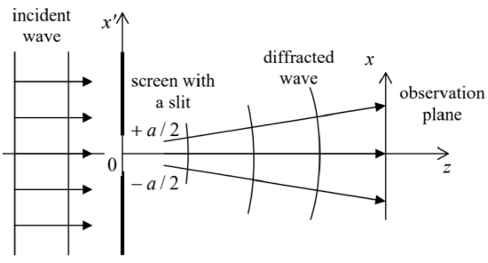Fig. 8.12. Diffraction on a slit.

Let us apply Eq. (91) to our current problem (Fig. 12), for the sake of simplicity assuming the normal wave incidence, and taking \(\ z^{\prime}=0\) at the screen plane:

\[\ f_{\omega}(x, z)=f_{0} \frac{k}{2 \pi i} \int_{-a}^{+a} d x^{\prime} \int_{-\infty}^{+\infty} d y^{\prime} \frac{\exp \left\{i k\left[\left(x-x^{\prime}\right)^{2}+y^{\prime 2}+z^{2}\right]^{1 / 2}\right\}}{\left[\left(x-x^{\prime}\right)^{2}+y^{\prime 2}+z^{2}\right]^{1 / 2}},\tag{8.104}\]

where \(\ f_{0} \equiv f_{\omega}\left(x^{\prime}, 0\right)=\text { const }\) is the incident wave’s amplitude. This is the same integral as in Eq. (85), except for the finite limits for the integration variable \(\ x^{\prime}\), and may be simplified similarly, using the small-angle condition \(\ \left(x-x^{\prime}\right)^{2}+y^{\prime 2}<<z^{2}\):

\[\ f_{\omega}(x, z) \approx f_{0} \frac{k}{2 \pi i} \frac{e^{i k z}}{z} \int_{-a / 2}^{+a / 2} d x^{\prime} \int_{-\infty}^{+\infty} d y^{\prime} \exp \frac{i k\left[\left(x-x^{\prime}\right)^{2}+y^{\prime 2}\right]}{2 z} \equiv f_{0} \frac{k}{2 \pi i} \frac{e^{i k z}}{z} I_{x} I_{y}.\tag{8.105}\]

The integral over \(\ y^{\prime}\) is the same as in the last section:

\[\ I_{y} \equiv \int_{-\infty}^{+\infty} \exp \frac{i k y^{\prime 2}}{2 z} d y^{\prime}=\left(\frac{2 \pi i z}{k}\right)^{1 / 2},\tag{8.106}\]

but the integral over \(\ x^{\prime}\) is more general, because of its finite limits:

\[\ I_{x} \equiv \int_{-a / 2}^{+a / 2} \exp \frac{i k\left(x-x^{\prime}\right)^{2}}{2 z} d x^{\prime}.\tag{8.107}\]

It may be simplified in the following two (opposite) limits.

(i) Fraunhofer diffraction takes place when \(\ z / a >> a / \lambda\) – the relation which may be rewritten either as \(\ a<<(z \lambda)^{1 / 2}\), or as \(\ k a^{2}<<z\). In this limit, the ratio \(\ k x^{, 2} / z\) is negligibly small for all values of \(\ x^{\prime}\) under the integral, and we can approximate it as

\[\ \begin{aligned}
I_{x} &=\int_{-a / 2}^{+a / 2} \exp \frac{i k\left(x^{2}-2 x x^{\prime}+x^{\prime 2}\right)}{2 z} d x^{\prime} \approx \int_{-a / 2}^{+a / 2} \exp \frac{i k\left(x^{2}-2 x x^{\prime}\right)}{2 z} d x^{\prime} \\
& \equiv \exp \frac{i k x^{2}}{2 z} \int_{-a / 2}^{+a / 2} \exp \left\{-\frac{i k x x^{\prime}}{z}\right\} d x^{\prime}=\frac{2 z}{k x} \exp \left\{\frac{i k x^{2}}{2 z}\right\} \sin \frac{k x a}{2 z},
\end{aligned}\tag{8.108}\]

so that Eq. (105) yields

\[\ f_{\omega}(x, z) \approx f_{0} \frac{k}{2 \pi i} \frac{e^{i k z}}{z} \frac{2 z}{k x}\left(\frac{2 \pi i z}{k}\right)^{1 / 2} \exp \left\{\frac{i k x^{2}}{2 z}\right\} \sin \frac{k x a}{2 z},\tag{8.109}\]

and hence the relative wave intensity is

\[\ \frac{\bar{S}(x, z)}{S_{0}}=\left|\frac{f_{\omega}(x, z)}{f_{0}}\right|^{2}=\frac{8 z}{\pi k x^{2}} \sin ^{2} \frac{k x a}{2 z} \equiv \frac{2}{\pi} \frac{k a^{2}}{z} \operatorname{sinc}^{2}\left(\frac{k a \theta}{2}\right),\quad\quad\quad\quad \text{Fraunhofer diffraction pattern}\tag{8.110}\]

where \(\ S_{0}\) is the intensity of the incident wave, and \(\ \theta \equiv x / z<<1\) is the observation angle. Comparing this expression with Eq. (69), we see that this diffraction pattern is exactly the same as that of a similar (uniform, 1D) object in the Born approximation – see the red line in Fig. 8. Note again that the angular width \(\ \delta \theta\) of the Fraunhofer pattern is of the order of \(\ 1/ka\), so that its linear width \(\ \delta x=z \delta \theta\) is of the order of \(\ z / k a \sim z \lambda / a\).⁴⁰ Hence the condition of the Fraunhofer approximation’s validity may be also represented as \(\ a<<\delta x\).

(ii) Fresnel diffraction. In the opposite limit of a relatively wide slit, with \(\ a>>\delta x=z\delta\theta\sim z/ka\sim z \lambda /a \text {, i.e. } k a^{2} >>z\), the diffraction patterns at two edges of the slit are well separated. Hence, near each edge (for example, near \(\ x^{\prime}=-a / 2\)) we may simplify Eq. (107) as

\[\ I_{x}(x) \approx \int_{-a / 2}^{+\infty} \exp \frac{i k\left(x-x^{\prime}\right)^{2}}{2 z} d x^{\prime} \equiv\left(\frac{2 z}{k}\right)^{1 / 2} \int_{(k / 2 z)^{1 / 2}(x+a / 2)}^{+\infty} \exp \left\{i \zeta^{2}\right\} d \zeta,\tag{8.111}\]

and express it via the special functions called the Fresnel integrals:⁴¹

\[\ \mathscr{C}(\xi) \equiv\left(\frac{2}{\pi}\right)^{1 / 2} \int_{0}^{\xi} \cos \left(\zeta^{2}\right) d \zeta, \quad \mathscr{S}(\xi) \equiv\left(\frac{2}{\pi}\right)^{1 / 2} \int_{0}^{\xi} \sin \left(\zeta^{2}\right) d \zeta,\quad\quad\quad\quad\text{Fresnel integrals}\tag{8.112}\]

whose plots are shown in Fig. 13a. As was mentioned above, at large values of their argument \(\ (\xi)\), both functions tend to 1⁄2.

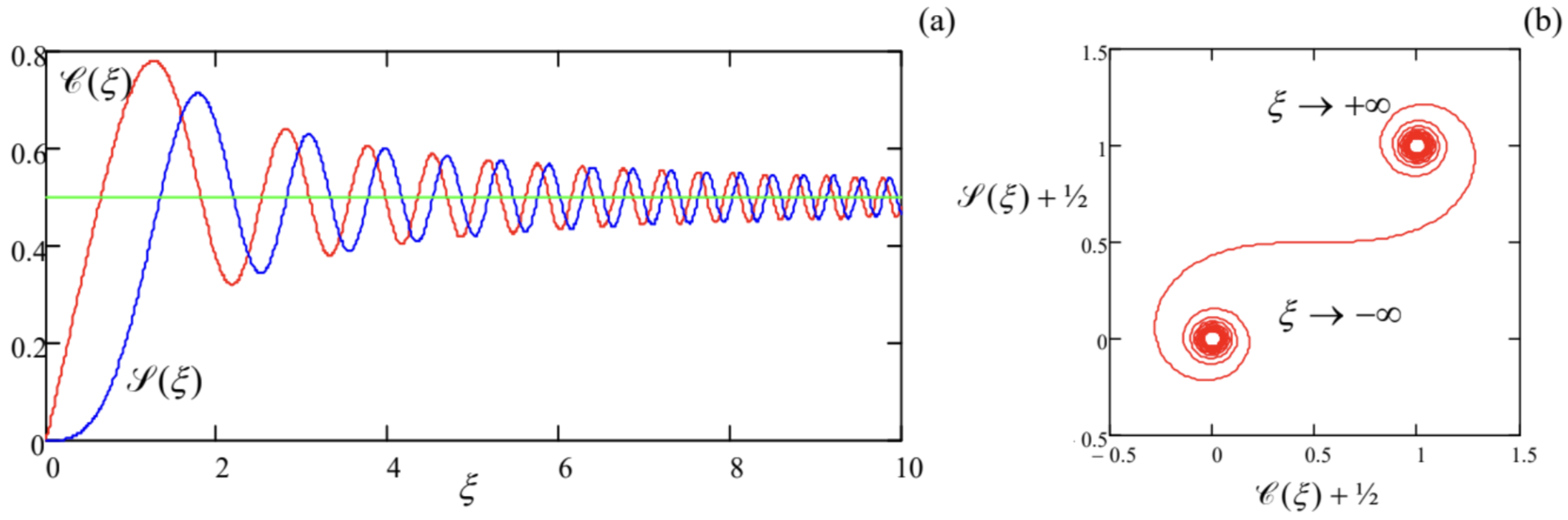Fig. 8. 13. (a) The Fresnel integrals and (b) their parametric representation.

Plugging this expression into Eqs. (105) and (111), for the diffracted wave intensity, in the Fresnel limit (i.e. at \(\ |x+a / 2|<<a\)), we get

\[\ \text{Fresnel diffraction pattern}\quad\quad\quad\quad \frac{\bar{S}(x, z)}{S_{0}}=\frac{1}{2}\left\{\left[\mathscr{C}\left(\left(\frac{k}{2 z}\right)^{1 / 2}\left(x+\frac{a}{2}\right)\right)+\frac{1}{2}\right]^{2}+\left[\mathscr{S}\left(\left(\frac{k}{2 z}\right)^{1 / 2}\left(x+\frac{a}{2}\right)\right)+\frac{1}{2}\right]^{2}\right\}.\tag{8.113}\]

A plot of this function (Fig. 14) shows that the diffraction pattern is very peculiar: while in the “shade” region \(\ x<-a / 2\) the wave intensity fades monotonically, the transition to the “light” region within the gap \(\ (x>-a / 2)\) is accompanied by intensity oscillations, just as at the Fraunhofer diffraction – cf. Fig. 8.

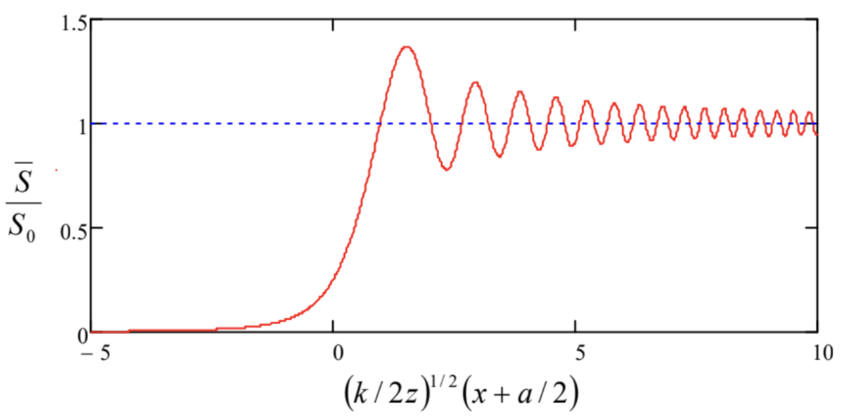Fig. 8.14. The Fresnel diffraction pattern.

This behavior, which is described by the following asymptotes,

\[\ \frac{\bar{S}}{S_{0}} \rightarrow \begin{cases}1+\frac{1}{\sqrt{\pi}} \frac{\sin \left(\xi^{2}-\pi / 4\right)}{\xi}, & \text { for } \xi \equiv\left(\frac{k}{2 z}\right)^{1 / 2}\left(x+\frac{a}{2}\right) \rightarrow+\infty, \\ \frac{1}{4 \pi \xi^{2}}, & \text { for } \xi \rightarrow-\infty,\end{cases}\tag{8.114}\]

is essentially an artifact of “observing” just the wave intensity (i.e. its real amplitude) rather than its phase as well. Indeed, as may be seen even more clearly from the parametric presentation of the Fresnel integrals, shown in Fig. 13b, these functions oscillate similarly at large positive and negative values of their argument. (This famous pattern is called either the Euler spiral or the Cornu spiral.) Physically, this means that the wave diffraction at the slit edge leads to similar oscillations of its phase at \(\ x<-a / 2\) and \(\ x>-a / 2\); however, in the latter region (i.e. inside the slit) the diffracted wave overlaps the incident wave passing through the slit directly, and their interference reveals the phase oscillations, making them visible in the measured intensity as well.

Note that according to Eq. (113), the linear scale \(\ \delta x\) of the Fresnel diffraction pattern is of the order of \(\ (2 z / k)^{1 / 2}\), i.e. is complies with the estimate given by Eq. (90). If the slit is gradually narrowed so that its width a becomes comparable to \(\ \delta x\),⁴² the Fresnel diffraction patterns from both edges start to “collide” (interfere). The resulting wave, fully described by Eq. (107), is just a sum of two contributions of the type (111) from both edges of the slit. The resulting interference pattern is somewhat complicated, and only when a becomes substantially less than \(\ \delta x\), it is reduced to the simple Fraunhofer pattern (110).

Of course, this crossover from the Fresnel to Fraunhofer diffraction may be also observed, at fixed wavelength \(\ \lambda\) and slit width \(\ a\), by increasing \(\ z\), i.e. by measuring the diffraction pattern farther and
farther away from the slit.

Note also that the Fraunhofer limit is always valid if the diffraction is measured as a function of the diffraction angle \(\ \theta\) alone. This may be done, for example, by collecting the diffracted wave with a “positive” (converging) lens and observing the diffraction pattern in its focal plane.

---

Reference

⁴⁰ Note also that since in this limit \(\ k a^{2}<<z\), Eq. (97) shows that even the maximum value \(\ S(0, z)\) of the diffracted wave’s intensity is much lower than that \(\ \left(S_{0}\right)\) of the incident wave. This is natural because the incident power \(\ S_{0} a\) per unit length of the slit is now distributed over a much larger width \(\ \delta x >> a\), so that \(\ S(0, z) \sim S_{0}(a / \delta x)<<S_{0}\).

⁴¹ Slightly different definitions of these functions, affecting the constant factors, may also be met in literature.

⁴² Note that this condition may be also rewritten as \(\ a \sim \delta x\), i.e. \(\ z / a \sim a / \lambda\).