2.8: Periodic Systems- Energy Bands and Gaps

Let us now proceed to the discussion of one of the most important issues of wave mechanics: particle motion through a periodic system. As a precursor to this discussion, let us calculate the transparency of the potential profile shown in Fig. 22 (frequently called the $\operatorname{Dirac}$ comb): a sequence of $N$ similar, equidistant delta-functional potential barriers, separated by $(N-1)$ potential-free intervals $a$.

Fig. 2.22. Tunneling through a Dirac comb: a system of $N$ similar, equidistant barriers, i.e. $(N-1)$ similar coupled potential wells.

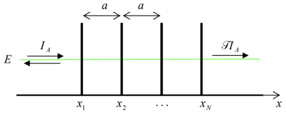
According to Eq. (132), its transfer matrix is the following product $$\mathrm{T}=\underbrace{\mathrm{T}_{\alpha} \mathrm{T}_{a} \mathrm{~T}_{\alpha} \ldots \mathrm{T}_{a} \mathrm{~T}_{\alpha}}_{(N-1)+N \text { terms }},$$ with the component matrices given by Eqs. (135) and (138), and the barrier height parameter $\alpha$ defined by the last of Eqs. (78). Remarkably, this multiplication may be carried out analytically, ${ }^{47}$ giving $$\mathscr{T} \equiv\left|T_{11}\right|^{-2}=\left[(\cos N q a)^{2}+\left(\frac{\sin k a-\alpha \cos k a}{\sin q a} \sin N q a\right)^{2}\right]^{-1},$$ where $q$ is a new parameter, with the wave number dimensionality, defined by the following relation: $$\cos q a \equiv \cos k a+\alpha \sin k a .$$ For $N=1$, Eqs. (191) immediately yield our old result (79), while for $N=2$ they may be readily reduced to Eq. (141) - see Fig. 16a. Fig. 20 shows its predictions for two larger numbers $N$, and several values of the dimensionless parameter $\alpha$.

Let us start the discussion of the plots from the case $N=3$, when three barriers limit two coupled potential wells between them. Comparison of Fig. 23a and Fig. 16 a shows that the transmission patterns, and their dependence on the parameter $\alpha$, are very similar, besides that in the coupled-well system, each resonant tunneling peak splits into two, with the $k a$-difference between them scaling as $1 / \alpha$. From the discussion in the last section, we may now readily interpret this result: each pair of resonance peaks of transparency corresponds to the alignment of the incident particle’s energy $E$ with the pair of energy levels $E_{\mathrm{A}}, E_{\mathrm{S}}$ of the symmetric and antisymmetric states of the system. However, in contrast to the system shown in Fig. 19, these states are metastable, because the particle may leak out from these states just as it could in the system studied in Sec. 5 - see Fig. 15 and its discussion. As a result, each of the resonant peaks has a non-zero energy width $\Delta E$, obeying Eq. (155).

Fig. 2.23. The Dirac comb’s transparency as a function of the product $k a$ for three values of $\alpha$. Since the function $\mathscr{T} k a$ ) is $\pi$-periodic (just like it is for $N=2$, see Fig. 16a), only one period is shown.

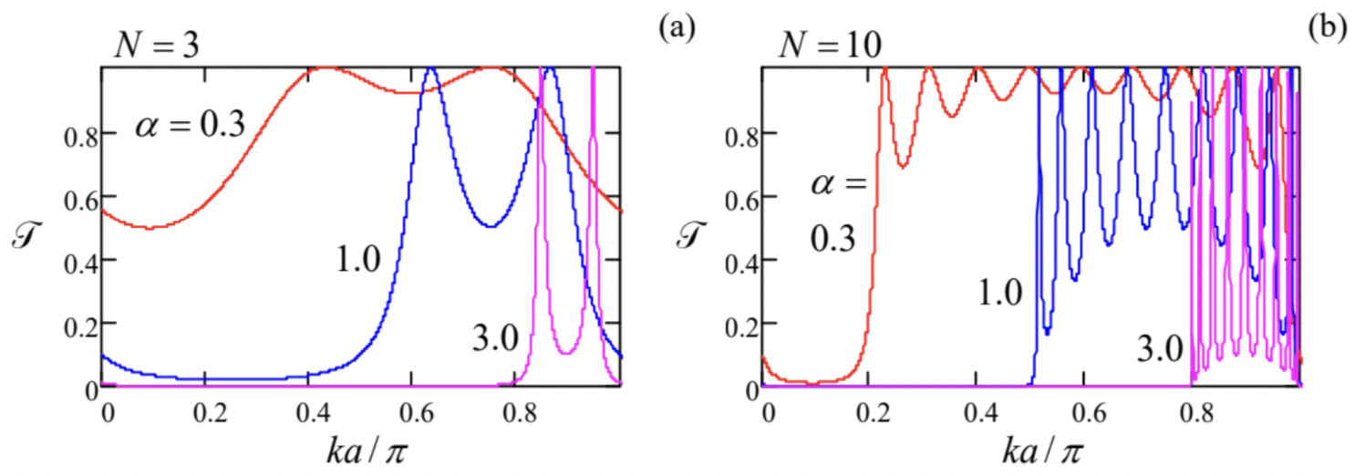
A further increase of $N$ (see Fig. 23b) results in the increase of the number of resonant peaks per period to $(N-1)$, and at $N \rightarrow \infty$ the peaks merge into the so-called allowed energy bands (frequently called just the "energy bands") with average transparency $\mathscr{T} \sim 1$, separated from similar bands in the adjacent periods of function $\mathcal{T}(\mathrm{ka})$ by energy gaps $^{48}$ where $\mathcal{T} \rightarrow 0$. Notice the following important features of the pattern:

(i) at $N \rightarrow \infty$, the band/gap edges become sharp for any $\alpha$, and tend to fixed positions (determined by $\alpha$ but independent of $N$ );

(ii) the larger is well coupling (the smaller is $\alpha$ ), the broader are the allowed energy bands and the narrower are the gaps between them.

Our previous discussion of the resonant tunneling gives us a clue for a semi-quantitative interpretation of this pattern: if $(N-1)$ potential wells are weakly coupled by tunneling through the potential barriers separating them, the system’s energy spectrum consists of groups of $(N-1)$ metastable energy levels, each group being close to one of the unperturbed eigenenergies of the well. (According to Eq. (1.84), for our current example shown in Fig. 22, with its rectangular potential wells, these eigenenergies correspond to $k_{n} a=\pi n$.)

Now let us recall that in the case $N=2$, analyzed in the previous section, the eigenfunctions (169) and (175) differed only by the phase shift $\Delta \varphi$ between their localized components $\psi_{\mathrm{R}}(x)$ and $\psi_{\mathrm{L}}(x)$, with $\Delta \varphi=0$ for one of them $(\psi \mathrm{s})$ and $\Delta \varphi=\pi$ for its counterpart. Hence it is natural to expect that for other $N$ as well, each metastable energy level corresponds to an eigenfunction that is a superposition of similar localized functions in each potential well, but with certain phase shifts $\Delta \varphi$ between them.

Moreover, we may expect that at $N \rightarrow \infty$, i.e. for periodic structures ${ }^{49}$ with $$U(x+a)=U(x),$$ when the system does not have the ends that could affect its properties, the phase shifts $\Delta \varphi$ between the localized wavefunctions in all couples of adjacent potential wells should be equal, i.e. $$\psi(x+a)=\psi(x) e^{i \Delta \varphi}$$ for all $x .{ }^{50}$ This equality is the (1D version of the) much-celebrated Bloch theorem. ${ }^{51}$ Mathematical rigor aside, ${ }^{52}$ it is a virtually evident fact because the particle’s density $w(x)=\psi^{*}(x) \psi(x)$, which has to be periodic in this $a$-periodic system, may be so only $\Delta \varphi$ is constant. For what follows, it is more convenient to represent the real constant $\Delta \varphi$ in the form $q a$, so that the Bloch theorem takes the form $$\psi(x+a)=\psi(x) e^{i q a} .$$ The physical sense of the parameter $q$ will be discussed in detail below, but we may immediately notice that according to Eq. (193b), an addition of $(2 \pi / a)$ to this parameter yields the same wavefunction; hence all observables have to be $(2 \pi / a)$-periodic functions of $q .{ }^{53}$

Now let us use the Bloch theorem to calculate the eigenfunctions and eigenenergies for the infinite version of the system shown in Fig. 22, i.e. for an infinite set of delta-functional potential barriers - see Fig. $24 .$

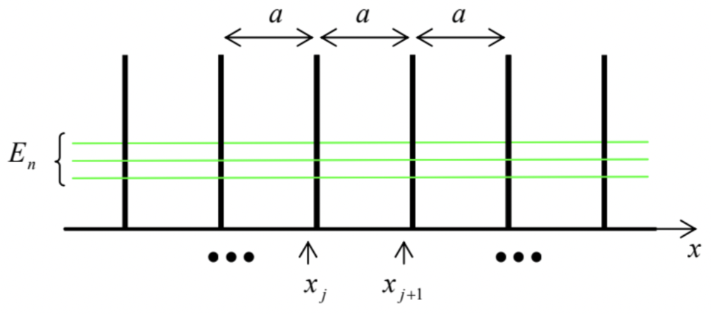Fig. 2.24. The simplest periodic potential: an infinite Dirac comb.

To start, let us consider two points separated by one period $a$ : one of them, $x_{j}$, just left of the position of one of the barriers, and another one, $x_{j+1}$, just left of the following barrier-see Fig. 24 again. The eigenfunctions at each of the points may be represented as linear superpositions of two simple waves $\exp \{\pm i k x\}$, and the amplitudes of their components should be related by a $2 \times 2$ transfer matrix $\mathrm{T}$ of the potential fragment separating them. According to Eq. (132), this matrix may be found as the product of the matrix (135) of one delta-functional barrier by the matrix (138) of one zero-potential interval $a$ : $$\left(\begin{array}{l} A_{j+1} \\ B_{j+1} \end{array}\right)=\mathrm{T}_{\mathbf{a}} \mathrm{T}_{\alpha}\left(\begin{array}{l} A_{j} \\ B_{j} \end{array}\right)=\left(\begin{array}{cc} e^{i k a} & 0 \\ 0 & e^{-i k a} \end{array}\right)\left(\begin{array}{cc} 1-i \alpha & -i \alpha \\ i \alpha & 1+i \alpha \end{array}\right)\left(\begin{array}{l} A_{j} \\ B_{j} \end{array}\right) .$$ However, according to the Bloch theorem (193b), the component amplitudes should be also related as $$\left(\begin{array}{l} A_{j+1} \\ B_{j+1} \end{array}\right)=e^{i q a}\left(\begin{array}{l} A_{j} \\ B_{j} \end{array}\right) \equiv\left(\begin{array}{cc} e^{i q a} & 0 \\ 0 & e^{i q a} \end{array}\right)\left(\begin{array}{l} A_{j} \\ B_{j} \end{array}\right) .$$ The condition of self-consistency of these two equations gives the following characteristic equation: $$\left|\left(\begin{array}{cc} e^{i k a} & 0 \\ 0 & e^{-i k a} \end{array}\right)\left(\begin{array}{cc} 1-i \alpha & -i \alpha \\ i \alpha & 1+i \alpha \end{array}\right)-\left(\begin{array}{cc} e^{i q a} & 0 \\ 0 & e^{i q a} \end{array}\right)\right|=0 .$$ In Sec. 5, we have already calculated the matrix product participating in this equation - see the second operand in Eq. (140). Using it, we see that Eq. (196) is reduced to the same simple Eq. (191b) that has jumped at us from the solution of the somewhat different (resonant tunneling) problem. Let us explore that simple result in detail. First of all, the left-hand side of Eq. (191b) is a sinusoidal function of the product $q a$ with unit amplitude, while its right-hand side is a sinusoidal function of the product $k a$, with amplitude $\left(1+\alpha^{2}\right)^{1 / 2}>1$ - see Fig. 25,

Fig. 2.25. The graphical representation of the characteristic equation (191b) for a fixed value of the parameter $\alpha$. The ranges of $k a$ that yield $|\cos q a|<1$, correspond to allowed energy bands, while those with $|\cos q a|>1$, correspond to energy gaps between them.

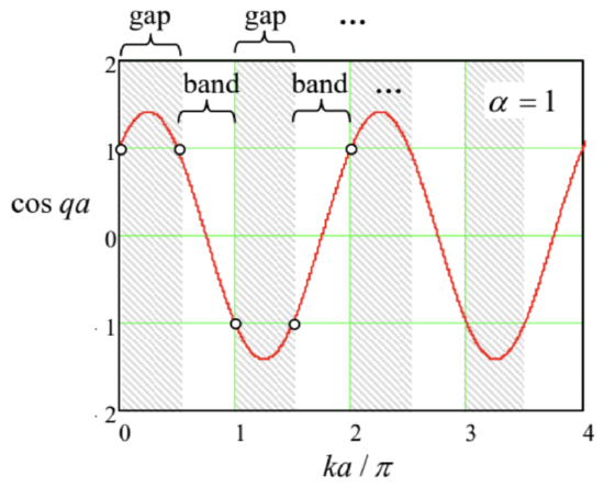
As a result, within each half-period $\Delta(k a)=\pi$ of the right-hand side, there is an interval where the magnitude of the right-hand side is larger than 1 , so that the characteristic equation does not have a real solution for $q$. These intervals correspond to the energy gaps (see Fig. 23 again), while the complementary intervals of $k a$, where a real solution for $q$ exists, correspond to the allowed energy bands. In contrast, the parameter $q$ can take any real values, so it is more convenient to plot the eigenenergy $E=\hbar^{2} k^{2} / 2 m$ as the function of the quasimomentum $\hbar q$ (or, even more conveniently, of the dimensionless parameter $q a$ ) rather than $k a .^{54}$ Before doing that, we need to recall that the parameter $\alpha$, defined by the last of Eqs. (78), depends on the wave vector $k$ as well, so that if we vary $q$ (and hence $k$ ), it is better to characterize the structure by another, $k$-independent dimensionless parameter, for example $$\beta \equiv(k a) \alpha \equiv \frac{w}{\hbar^{2} / m a},$$ so that our characteristic equation (191b) becomes $$\cos q a \equiv \cos k a+\beta \frac{\sin k a}{k a} .$$ Fig. 26 shows the plots of $k$ and $E$, following from Eq. (198), as functions of $q a$, for a particular, moderate value of the parameter $\beta$. The first evident feature of the pattern is the $2 \pi$-periodicity of the pattern in the argument $q a$, which we have already predicted from the general Bloch theorem arguments. (Due to this periodicity, the complete band/gap pattern may be studied, for example, on just one interval $-\pi \leq q a \leq+\pi$, called the $1^{\text {st }}$ Brillouin zone - the so-called reduced zone picture. For some applications, however, it is more convenient to use the extended zone picture with $-\infty \leq q a \leq+\infty-$ see, e.g., the next section.)

Fig. 2.26. (a) The "genuine" momentum $k$ of a particle in an infinite Dirac comb (Fig. 24), and (b) its energy $E=\hbar^{2} k^{2} / 2 m$ (in the units of $E_{0} \equiv \hbar^{2} / 2 m a^{2}$ ), as functions of normalized quasimomentum, for a particular value $(\beta=3)$ of the dimensionless parameter defined by Eq. (197). Arrows in the lower right corner of panel (b) illustrate the definition of energy band $\left(\Delta E_{n}\right)$ and energy gap $\left(\Delta_{n}\right)$ widths.

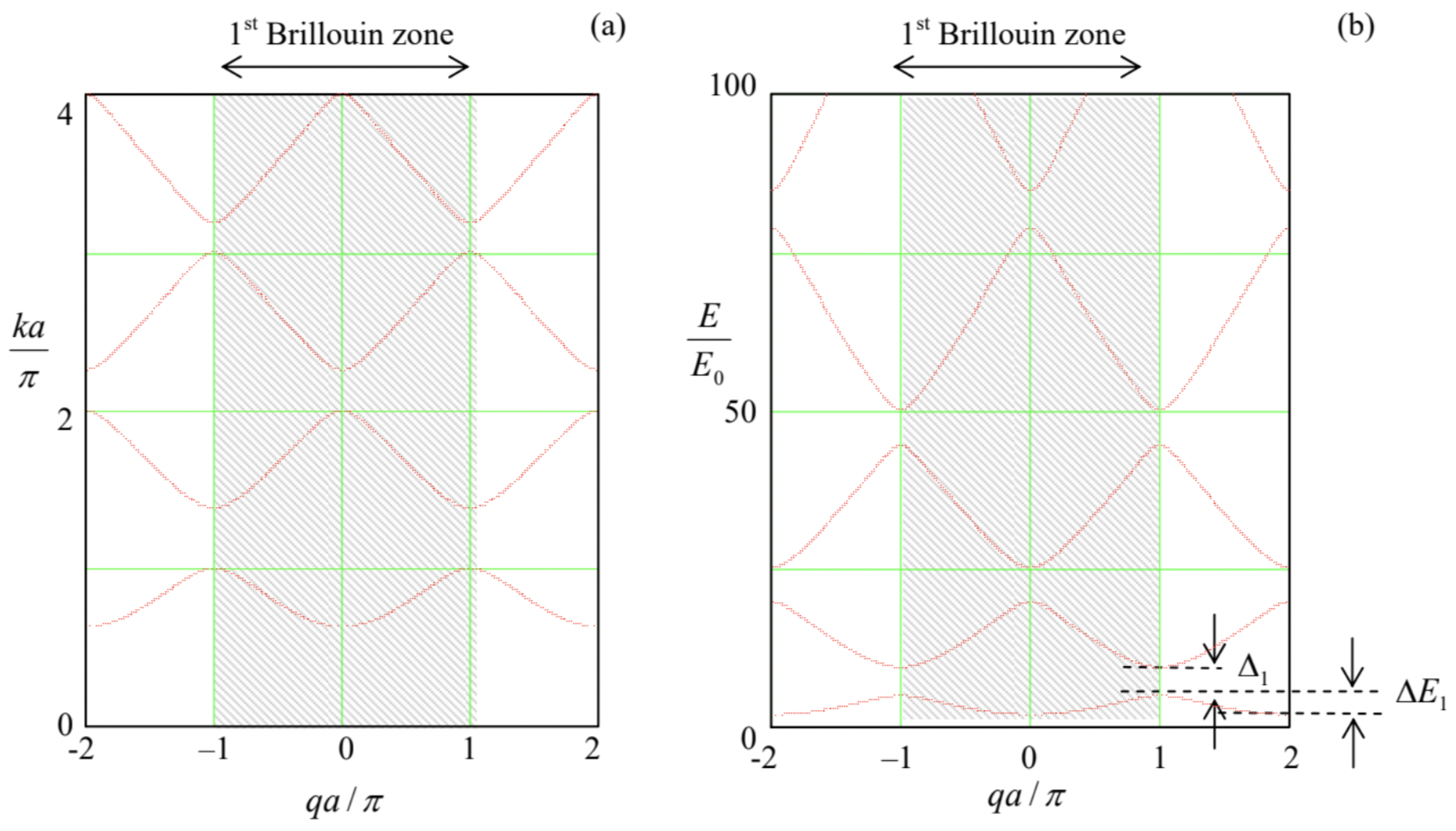
However, maybe the most important fact, clearly visible in Fig. 26, is that there is an infinite number of energy bands, with different energies $E_{n}(q)$ for the same value of $q$. Mathematically, it is evident from Eq. (198) - or alternatively from Fig. 25. Indeed, for each value of $q a$, there is a solution $k a$ to this equation on each half-period $\Delta(k a)=\pi$. Each of such solutions (see Fig. 26a) gives a specific value of particle’s energy $E=\hbar^{2} k^{2} / 2 m$. A continuous set of similar solutions for various $q a$ forms a particular energy band.

Since the energy band picture is one of the most practically important results of quantum mechanics, it is imperative to understand its physics. It is natural to describe this physics in two different ways in two opposite potential strength limits. In parallel, we will use this discussion to obtain simpler expressions for the energy band/gap structure in each limit. An important advantage of this approach is that both analyses may be carried out for an arbitrary periodic potential $U(x)$ rather than for the particular model shown in Fig. 24 .

(i) Tight-binding approximation. This approximation works well when the eigenenergy $E_{n}$ of the states quasi-localized at the energy profile minima is much lower than the height of the potential barriers separating them - see Fig. 27. As should be clear from our discussion in Sec. 6, essentially the only role of coupling between these states (via tunneling through the potential barriers separating the minima) is to establish a certain phase shift $\Delta \varphi \equiv q a$ between the adjacent quasi-localized wavefunctions $u_{n}\left(x-x_{j}\right)$ and $u_{n}\left(x-x_{j+1}\right)$.

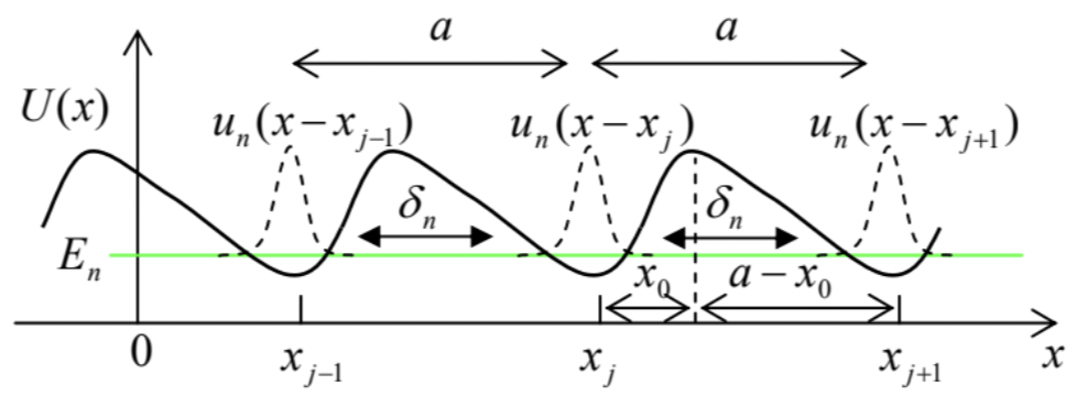Fig. 2. 27. The tight-binding approximation (schematically).

To describe this effect quantitatively, let us first return to the problem of two coupled wells considered in Sec. 6 , and recast the result $(180)$, with restored eigenstate index $n$, as $$\Psi_{n}(x, t)=\left[a_{\mathrm{R}}(t) \psi_{\mathrm{R}}(x)+a_{\mathrm{L}}(t) \psi_{\mathrm{L}}(x)\right] \exp \left\{-i \frac{E_{n}}{\hbar} t\right\},$$ where the probability amplitudes $a_{\mathrm{R}}$ and $a_{\mathrm{L}}$ oscillate sinusoidally in time: $$a_{\mathrm{R}}(t)=\cos \frac{\delta_{n}}{\hbar} t, \quad a_{\mathrm{L}}(t)=i \sin \frac{\delta_{n}}{\hbar} t .$$ This evolution satisfies the following system of two equations whose structure is similar to Eq. (1.61a): $$i \hbar \dot{a}_{\mathrm{R}}=-\delta_{n} a_{\mathrm{L}}, \quad i \hbar \dot{a}_{\mathrm{L}}=-\delta_{n} a_{\mathrm{R}} .$$ Eq. (199) may be readily generalized to the case of many similar coupled wells: $$\Psi_{n}(x, t)=\left[\sum_{j} a_{j}(t) u_{n}\left(x-x_{j}\right)\right] \exp \left\{-i \frac{E_{n}}{\hbar} t\right\},$$ where $E_{n}$ are the eigenenergies and $u_{n}$ the eigenfunctions of each well. In the tight-binding limit, only the adjacent wells are coupled, so that instead of Eq. (201) we should write an infinite system of similar equations $$i \hbar \dot{a}_{j}=-\delta_{n} a_{j-1}-\delta_{n} a_{j+1},$$ for each well number $j$, where parameters $\delta_{n}$ describe the coupling between two adjacent potential wells. Repeating the calculation outlined at the end of the last section for our new situation, for a smooth potential we may get an expression essentially similar to the last form of Eq. (188): $$\delta_{n}=\frac{\hbar^{2}}{m} u_{n}\left(x_{0}\right) \frac{d u_{n}}{d x}\left(a-x_{0}\right)$$ where $x_{0}$ is the distance between the well bottom and the middle of the potential barrier on the right of it - see Fig. 27. The only substantial new feature of this expression in comparison with Eq. (188) is that the sign of $\delta_{n}$ alternates with the level number $n: \delta_{1}>0, \delta_{2}<0, \delta_{3}>0$, etc. Indeed, the number of zeros (and hence, "wiggles") of the eigenfunctions $u_{n}(x)$ of any potential well increases as $n-$ see, e.g., Fig. $1.8{ }^{55}$ so that the difference of the exponential tails of the functions, sneaking under the left and right barriers limiting the well also alternates with $n$.

The infinite system of ordinary differential equations (203) enables solutions of many important problems (such as the spread of the wavefunction that was initially localized in one well, etc.), but our task right now is just to find its stationary states, i.e. the solutions proportional to $\exp \left\{-i\left(\varepsilon_{n} / \hbar\right) t\right\}$, where $\varepsilon_{n}$ is a still unknown, $q$-dependent addition to the background energy $E_{n}$ of the $n^{\text {th }}$ energy level. To satisfy the Bloch theorem (193) as well, such a solution should have the following form: $$a_{j}(t)=a \exp \left\{i q x_{j}-i \frac{\varepsilon_{n}}{\hbar} t+\text { const }\right\} .$$ Plugging this solution into Eq. (203) and canceling the common exponent, we get $$E=E_{n}+\varepsilon_{n}=E_{n}-\delta_{n}\left(e^{-i q a}+e^{i q a}\right) \equiv E_{n}-2 \delta_{n} \cos q a$$ so that in this approximation, the energy band width $\Delta E_{n}$ (see Fig. 26b) equals $4\left|\delta_{n}\right|$.

The relation (206), whose validity is restricted to $\left|\delta_{n}\right|<<E_{n}$, describes the lowest energy bands plotted in Fig. 26b reasonably well. (For larger $\beta$, the agreement would be even better.) So, this calculation explains what the energy bands really are: in the tight-binding limit they are best interpreted as isolated well’s energy levels $E_{n}$, broadened into bands by the interwell interaction. Also, this result gives clear proof that the energy band extremes correspond to $q a=2 \pi l$ and $q a=2 \pi(l+1 / 2)$, with integer l. Finally, the sign alteration of the coupling coefficient $\delta_{n}(204)$ explains why the energy maxima of one band are aligned, on the $q a$ axis, with energy minima of the adjacent bands - see Fig. 26 .

(ii) Weak-potential limit. Amazingly, the energy-band structure is also compatible with a completely different physical picture that may be developed in the opposite limit. Let the particle’s energy $E$ be so high that the periodic potential $U(x)$ may be treated as a small perturbation. Naively, in this limit we could expect a slightly and smoothly deformed parabolic dispersion relation $E=\hbar^{2} k^{2} / 2 m$. However, if we are plotting the stationary-state energy as a function of $q$ rather than $k$, we need to add $2 \pi l / a$, with an arbitrary integer $l$, to the argument. Let us show this by expanding all variables into the 1D-spatial Fourier series. For the potential energy $U(x)$ that obeys Eq. (192), such an expansion is straightforward: 56 $$U(x)=\sum_{l^{\prime \prime}} U_{l^{\prime}} \exp \left\{-i \frac{2 \pi x}{a} l^{\prime \prime}\right\}$$ where the summation is over all integers $l$ ", from $-\infty$ to $+\infty$. However, for the wavefunction we should show due respect to the Bloch theorem (193), which shows that strictly speaking, $\psi(x)$ is not periodic.

To overcome this difficulty, let us define another function: $$u(x) \equiv \psi(x) e^{-i q x},$$ and study its periodicity: $$u(x+a)=\psi(x+a) e^{-i q(x+a)}=\psi(x) e^{-i q x}=u(x)$$ We see that the new function is $a$-periodic, and hence we can use Eqs. (208)-(209) to rewrite the Bloch theorem in a different form: $$\psi(x)=u(x) e^{i q x}, \text { with } u(x+a)=u(x) .$$ Now it is safe to expand the periodic function $u(x)$ exactly as $U(x)$ : $$u(x)=\sum_{l^{\prime}} u_{l} \exp \left\{-i \frac{2 \pi x}{a} l^{\prime}\right\},$$ so that, according to Eq. (210), $$\psi(x)=e^{i q x} \sum_{l^{\prime}} u_{l^{\prime}} \exp \left\{-i \frac{2 \pi x}{a} l^{\prime}\right\}=\sum_{l^{\prime}} u_{l^{\prime}} \exp \left\{i\left(q-\frac{2 \pi}{a} l^{\prime}\right) x\right\} .$$ The only nontrivial part of plugging Eqs. (207) and (212) into the stationary Schrödinger equation (53) is how to handle the product term, $$U(x) \psi=\sum_{l^{\prime}, l^{\prime \prime}} U_{l^{\prime} u} u_{l^{\prime}} \exp \left\{\left[i\left[q-\frac{2 \pi}{a}\left(l^{\prime}+l^{\prime \prime}\right)\right] x\right\} .\right.$$ At fixed $l^{\prime}$, we may change the summation over $l$ " to that over $l \equiv l^{\prime}+l^{\prime \prime}$ (so that $l^{\prime \prime} \equiv l-l^{\prime}$ ), and write: $$U(x) \psi=\sum_{l} \exp \left\{i\left(q-\frac{2 \pi}{a} l\right) x\right\} \sum_{l^{\prime}} u_{l^{\prime}} U_{l-l^{\prime}} .$$ Now plugging Eq. (212) (with the summation index $l$ ’ replaced with $l$ ) and Eq. (214) into the stationary Schrödinger equation (53), and requiring the coefficients of each spatial exponent to match, we get an infinite system of linear equations for $u_{l}$ :

$$\sum_{l^{\prime}} U_{l-l^{\prime}} u_{l^{\prime}}=\left[E-\frac{\hbar^{2}}{2 m}\left(q-\frac{2 \pi}{a} l\right)^{2}\right] u_{l} .$$ (Note that by this calculation we have essentially proved that the Bloch wavefunction (210) is indeed $a$ solution of the Schrödinger equation, provided that the quasimomentum $q$ is selected in a way to make the system of linear equation (215) compatible, i.e. is a solution of its characteristic equation.)

So far, the system of equations (215) is an equivalent alternative to the initial Schrödinger equation, for any potential’s strength. ${ }^{57}$ In the weak-potential limit, i.e. if all Fourier coefficients $U_{n}$ are small ${ }^{58}$ we can complete all the calculations analytically. ${ }^{59}$ Indeed, in the so-called $0^{\text {th }}$ approximation we can ignore all $U_{n}$, so that in order to have at least one $u_{l}$ different from 0 , Eq. (215) requires that $$E \rightarrow E_{l} \equiv \frac{\hbar^{2}}{2 m}\left(q-\frac{2 \pi l}{a}\right)^{2} .$$ ( $u_{l}$ itself should be obtained from the normalization condition). This result means that in this approximation, the dispersion relation $E(q)$ has an infinite number of similar quadratic branches numbered by integer $l$ - see Fig. 28 .

Fig. 2.28. The energy band/gap picture in the weak potential limit $\left(\Delta_{n}\right.$ $<<E^{(n)}$ ), with the shading showing the $1^{\text {st }}$ Brillouin zone.

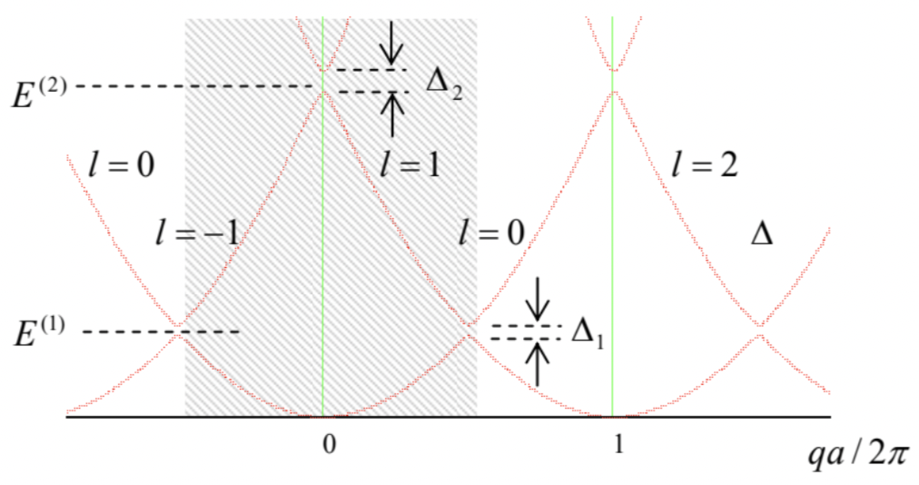
On every branch, such eigenfunction has just one Fourier coefficient, i.e. is a monochromatic traveling wave $$\psi_{l} \rightarrow u_{l} e^{i k x}=u_{l} \exp \left\{i\left(q-\frac{2 \pi l}{a}\right) x\right\} .$$ Next, the above definition of $E_{l}$ allows us to rewrite Eq. (215) in a more transparent form $$\sum_{l^{\prime} \neq l} U_{l-l^{\prime}} u_{l^{\prime}}=\left(E-E_{l}\right) u_{l},$$ which may be formally solved for $u_{l}$ : $$u_{l}=\frac{1}{E-E_{l}} \sum_{l^{\prime} \neq l} U_{l-l^{\prime}} u_{l^{\prime}}$$ This formula shows that if the Fourier coefficients $U_{n}$ are non-zero but small, the wavefunctions do acquire other Fourier components (besides the main one, with the index corresponding to the branch number), but these additions are all small, besides narrow regions near the points $E_{l}=E_{l}$, where two branches (216) of the dispersion relation $E(q)$, with some specific numbers $l$ and $l^{\prime}$, cross. According to Eq. (216), this happens when $$\left(q-\frac{2 \pi}{a} l\right) \approx-\left(q-\frac{2 \pi}{a} l^{\prime}\right),$$ i.e. at $q \approx q_{m} \equiv \pi m / a$ (with the integer $m \equiv l+l^{\prime}$ ) ${ }^{60}$ corresponding to $$E_{l} \approx E_{l} \approx \frac{\hbar^{2}}{2 m a^{2}}\left[\pi\left(l+l^{\prime}\right)-2 \pi l\right]^{2}=\frac{\pi^{2} \hbar^{2}}{2 m a^{2}} n^{2} \equiv E^{(n)},$$ with integer $n \equiv l-l^{\prime}$. (According to their definitions, the index $n$ is just the number of the branch crossing on the energy scale, while the index $m$ numbers the position of the crossing points on the $q$-axis - see Fig. 28.) In such a region, $E$ has to be close to both $E_{l}$ and $E_{l}$, so that the denominator in just one of the infinite number of terms in Eq. (219) is very small, making the term substantial despite the smallness of $U_{n}$. Hence we can take into account only one term in each of the sums (written for $l$ and $l^{\prime}$ ): $$\begin{aligned} &U_{n} u_{l^{\prime}}=\left(E-E_{l}\right) u_{l}, \\ &U_{-n} u_{l}=\left(E-E_{l^{\prime}}\right) u_{l^{\prime}} . \end{aligned}$$ Taking into account that for any real function $U(x)$, the Fourier coefficients in its Fourier expansion (207) have to be related as $U_{-n}=U_{n}{ }^{*}$, Eq. (222) yields the following simple characteristic equation $$\left|\begin{array}{cc} E-E_{l} & -U_{n} \\ -U_{n}^{*} & E-E_{l^{\prime}} \end{array}\right|=0,$$ with the following solution: $$E_{\pm}=E_{\text {ave }} \pm\left[\left(\frac{E_{l}-E_{l}}{2}\right)^{2}+U_{n} U_{n}^{*}\right]^{1 / 2}, \quad \text { with } E_{\text {ave }} \equiv \frac{E_{l}+E_{l^{\prime}}}{2}=E^{(n)}$$ According to Eq. (216), close to the branch crossing point $q_{m}=\pi\left(l+l^{\prime}\right) / a$, the fraction participating in this result may be approximated as ${ }^{61}$ $$\frac{E_{l}-E_{l^{\prime}}}{2} \approx \gamma \widetilde{q}, \quad \text { with }\left.\gamma \equiv \frac{d E_{l}}{d q}\right|_{q=q_{m}}=\frac{\pi \hbar^{2} n}{m a}=\frac{2 a E^{(n)}}{\pi n}, \quad \text { and } \widetilde{q} \equiv q-q_{m},$$ while the parameters $E_{\text {ave }}=E^{(n)}$ and $U_{n} U_{n}{ }^{*}=\left|U_{n}\right|^{2}$ do not depend on $\widetilde{q}$, i.e. on the distance from the central point $q_{m}$. This is why Eq. (224) may be plotted as the famous level anticrossing (also called "avoided crossing", or "intended crossing", or "non-crossing") diagram (Fig. 29), with the energy gap width $\Delta_{n}$ equal to $2\left|U_{n}\right|$, i.e. just twice the magnitude of the $n$-th Fourier harmonic of the periodic potential $U(x)$. Such anticrossings are also clearly visible in Fig. 28, which shows the result of the exact solution of Eq. (198) for the particular case $\beta=0.5 .62$

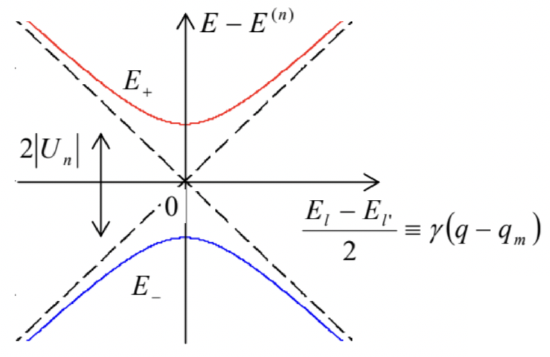Fig. 2.29. The level anticrossing diagram.

We will run into the anticrossing diagram again and again in the course, notably at the discussion of spin- $-\frac{2}{2}$ and other two-level systems. It is also repeatedly met in classical mechanics, for example at the calculation of frequencies of coupled oscillators. ${ }^{63} \cdot 64{ }^{4}$ In our current case of the weak potential limit of the band theory, the diagram describes the interaction of two traveling de Broglie waves (217), with oppositely directed wave vectors, $l$ and $-l^{\prime}$, via the $\left(l-l^{\prime}\right)^{\text {th }}$ (i.e. the $n^{\text {th }}$ ) Fourier harmonic of the potential profile $U(x){ }^{65}$ This effect exists also in the classical wave theory and is known as the Bragg reflection, describing, for example, the 1D model of the X-wave reflection by a crystal lattice (see, e.g. Fig. 1.5) in the limit of weak interaction between the incident wave and each atom.

The anticrossing diagram shows that rather counter-intuitively, even a weak periodic potential changes the topology of the initially parabolic dispersion relation radically, connecting its different branches, and thus creating the energy gaps. Let me hope that the reader has enjoyed the elegant description of this effect, discussed above, as well as one more illustration of the wonderful ability of physics to give completely different interpretations (and different approximate approaches) to the same effect in opposite limits.

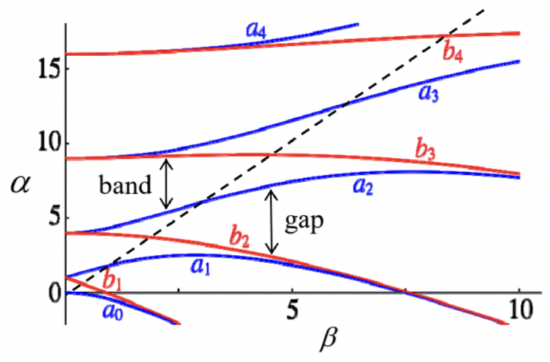
So, we have explained analytically (though only in two limits) the particular band structure shown in Fig. 26. Now we may wonder how general this structure is, i.e. how much of it is independent of the Dirac comb model (Fig. 24). For that, let us represent the band pattern, such as that shown in Fig. $26 \mathrm{~b}$ (plotted for a particular value of the parameter $\beta$, characterizing the potential barrier strength) in a more condensed form, which would allow us to place the results for a range of $\beta$ values on a single comprehensible plot. The way to do this should be clear from Fig. 26b: since the dependence of energy on the quasimomentum in each energy band is not too eventful, we may plot just the highest and the smallest values of the particle’s energy $E=\hbar^{2} k^{2} / 2 m$ as functions of $\beta \equiv$ maw/ $\hbar^{2}$ - see Fig. 30, which may be obtained from Eq. (198) with $q a=0$ and $q a=\pi$.

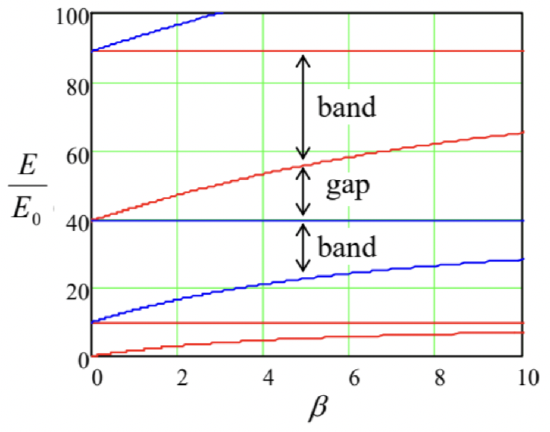Fig. 2.30. Characteristic curves of the Schrödinger equation for the infinite Dirac comb (Fig. 24).

These plots (in mathematics, commonly called characteristic curves, while in applied physics, band-edge diagrams) show, first of all, that at small $\beta$, all energy gap widths are equal and proportional to this parameter, and hence to $w$. This feature is in a full agreement with the main conclusion (224) of our general analysis of the weak-potential limit, because for the Dirac comb potential (Fig. 24), $$U(x)=w \sum_{j=-\infty}^{+\infty} \delta(x-j a+\text { const })$$ all Fourier harmonic amplitudes, defined by Eq. (207), are equal by magnitude: $\left|U_{l}\right|=W / a$. As $\beta$ is further increased, the gaps grow and the allowed energy bands shrink, but rather slowly. This is also natural, because, as Eq. (79) shows, transparency $\mathscr{T}$ of the delta-functional barriers separating the quasilocalized states (and hence the coupling parameters $\delta_{n} \propto \mathscr{T}^{/ 2}$ participating in the general tight-binding limit’s theory) decrease with $w \propto \beta$ very gradually.

These features may be compared with those for more realistic and relatively simple periodic functions $U(x)$, for example the sinusoidal potential $U(x)=A \cos (2 \pi x / a)-$ see Fig. 31a. For this potential, the stationary Schrödinger equation (53) takes the following form: $$-\frac{\hbar^{2}}{2 m} \frac{d^{2} \psi}{d x^{2}}+A \cos \frac{2 \pi x}{a} \psi=E \psi .$$ By introduction of dimensionless variables ${ }^{66}$ $$\xi \equiv \frac{\pi x}{a}, \quad \alpha \equiv \frac{E}{E^{(1)}}, \quad 2 \beta \equiv \frac{A}{E^{(1)}},$$ where $E^{(1)}$ is defined by Eq. (221) with $n=1$, Eq. (227) is reduced to the canonical form of the wellstudied Mathieu equation $^{67}$

Fig. 2.31. Two other simple periodic potential profiles: (a) the sinusoidal (“Mathieu”) potential and (b) the Kronig-Penney potential.

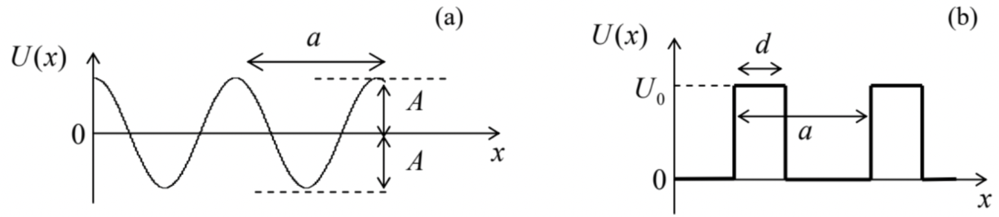
Fig. 2.31. Two other simple periodic potential profiles: (a) the sinusoidal ("Mathieu") potential and (b) the Kronig-Penney potential.

Figure 32 shows the characteristic curves of this equation. We see that now at small $\beta$ the first energy gap grows much faster than the higher ones: $\Delta_{n} \propto \beta^{n}$. This feature is in accord with the weakcoupling result $\Delta_{1}=2\left|U_{1}\right|$, which is valid only in the linear approximation in $U_{n}$, because for the Mathieu potential, $U_{l}=A\left(\delta_{l,+1}+\delta_{l,-1}\right) / 2$. Another clearly visible feature is the exponentially fast shrinkage of the allowed energy bands at $2 \beta>\alpha$ (in Fig. 32, on the right from the dashed line), i.e. at $E<A$. It may be readily explained by our tight-binding approximation result $(206)$ : as soon as the eigenenergy drops significantly below the potential maximum $U_{\max }=A$ (see Fig. 31a), the quantum states in the adjacent potential wells are connected only by tunneling through relatively high potential barriers separating these wells, so that the coupling amplitudes $\delta_{n}$ become exponentially small - see, e.g., Eq. (189).

Fig. 2.32. Characteristic curves of the Mathieu equation. The dashed line corresponds to the equality $\alpha=2 \beta$, i.e. $E$ $=A \equiv U_{\max }$, separating the regions of under-barrier tunneling and over-barrier motion. Adapted from Fig. 28.2.1 at http://dlmf.nist.gov. (Contribution by US Government, not subject to copyright).

Another simple periodic profile is the Kronig-Penney potential, shown in Fig. 31b, which gives relatively simple analytical expressions for the characteristic curves. Its advantage is a more realistic law of the decrease of the Fourier harmonics $U_{l}$ at $l \gg>1$, and hence of the energy gaps in the weak-potential limit:

$$\Delta_{n} \approx 2\left|U_{n}\right| \propto \frac{U_{0}}{n}, \text { at } E \sim E^{(n)} \gg U_{0} .$$ Leaving a detailed analysis of the Kronig-Penney potential for the reader’s exercise, let me conclude this section by addressing the effect of potential modulation on the number of eigenstates in 1D systems of a large but finite length $l \gg a, k^{-1}$. Surprisingly, the Bloch theorem makes the analysis of this problem elementary, for arbitrary $U(x)$. Indeed, let us assume that $l$ is comprised of an integer number of periods $a$, and its ends are described by similar boundary conditions - both assumptions evidently inconsequential for $l \gg>a$. Then, according to Eq. (210), the boundary conditions impose, on the quasimomentum $q$, exactly the same quantization condition as we had for $k$ for a free 1D motion. Hence, instead of Eq. (1.100), we can write $$d N=\frac{l}{2 \pi} d q,$$ with the corresponding change of the summation rule: $$\sum_{q} f(q) \rightarrow \frac{l}{2 \pi} \int f(q) d k .$$ As a result, the density of states in the $1 \mathrm{D}$ q-space, $d N / d q=l / 2 \pi$, does not depend on the potential profile at all! Note, however, that the profile does affect the density of states on the energy scale, $d N / d E$. As an extreme example, on the bottom and at the top of each energy band we have $d E / d q$ $\rightarrow 0$, and hence $$\frac{d N}{d E}=\frac{d N}{d q} / \frac{d E}{d q}=\frac{l}{2 \pi} / \frac{d E}{d q} \rightarrow \infty$$ This effect of state concentration at the band/gap edges (which survives in higher spatial dimensionalities as well) has important implications for the operation of several important electronic and optical devices, in particular semiconductor lasers and light-emitting diodes.

---

${ }^{47}$ This formula will be easier to prove after we have discussed the properties of Pauli matrices in Chapter $4 .$

${ }^{48}$ In solid-state (especially semiconductor) physics and electronics, the term bandgaps is more common.

${ }^{49}$ This is a reasonable 1D model, for example, for solid-state crystals, whose samples may feature up to $\sim 10^{9}$ similar atoms or molecules in each direction of the crystal lattice.

${ }^{50}$ A reasonably fair classical image of $\Delta \varphi$ is the geometric angle between similar objects - e.g., similar paper clips - attached at equal distances to a long, uniform rubber band. If the band’s ends are twisted, the twist is equally distributed between the structure’s periods, representing the constancy of $\Delta \varphi$. (I have to confess that, due to the lack of time, this was the only "lecture demonstration" in my Stony Brook QM courses.)

${ }^{51}$ Named after F. Bloch who applied this concept to the wave mechanics in 1929, i.e. very soon after its formulation. Note, however, that an equivalent statement in mathematics, called the Floquet theorem, has been known since at least 1883 .

${ }^{52}$ I will recover this rigor in two steps. Later in this section, we will see that the function obeying Eq. (193) is indeed $a$ solution to the Schrödinger equation. However, to save time/space, it will be better for us to postpone until Chapter 4 the proof that any eigenfunction of the equation, with periodic boundary conditions, obeys the Bloch theorem. As a partial reward for this delay, that proof will be valid for an arbitrary spatial dimensionality.

${ }^{53}$ The product $\hbar q$, which has the dimensionality of linear momentum, is called either the quasimomentum or (especially in solid-state physics) the "crystal momentum" of the particle. Informally, it is very convenient (and common) to use the name "quasimomentum" for the bare $q$ as well, despite its evidently different dimensionality.

${ }^{54}$ A more important reason for taking $q$ as the argument is that for a general periodic potential $U(x)$, the particle’s momentum $\hbar k$ is not uniquely related to $E$, while (according to the Bloch theorem) the quasimomentum $\hbar q$ is.

${ }^{55}$ Below, we will see several other examples of this behavior. This alternation rule is also described by the Wilson-Sommerfeld quantization condition (110).

${ }^{56}$ The benefits of such an unusual notation of the summation index ( $l$ " instead of, say, $l$ ) will be clear in a few lines.

${ }^{57}$ By the way, the system is very efficient for fast numerical solution of the stationary Schrödinger equation for any periodic profile $U(x)$, even though to describe potentials with large $U_{n}$, this approach may require taking into account a correspondingly large number of Fourier amplitudes $u_{l}$.

${ }^{58}$ Besides, possibly, a constant potential $U_{0}$, which, as was discussed in Chapter 1, may be always taken for the energy reference. As a result, in the following calculations, I will take $U_{0}=0$ to simplify the formulas.

${ }^{59}$ This method is so powerful that its multi-dimensional version is not much more complex than the 1D version described here - see, e.g., Sec. $3.2$ in the classical textbook by J. Ziman, Principles of the Theory of Solids, $2^{\text {nd }}$ ed., Cambridge U. Press, $1979 .$

${ }^{60}$ Let me hope that the difference between this new integer and the particle’s mass, both called $m$, is absolutely clear from the context.

${ }^{61}$ Physically, $\gamma \hbar \equiv \hbar(\pi n / a) / m=\hbar k^{(n)} / m$ is just the velocity of a free classical particle with energy $E^{(n)}$.

${ }^{62}$ From that figure, it is also clear that in the weak potential limit, the width $\Delta E_{n}$ of the $n^{\text {th }}$ energy band is just $E^{(n)}$ $-E^{(n-1)}-$ see Eq. (221). Note that this is exactly the distance between the adjacent energy levels of the simplest 1D potential well of infinite depth $-$ cf. Eq. (1.85).

${ }^{63}$ See, e.g., CM Sec. $6.1$ and in particular Fig. $6.2$.

${ }^{64}$ Actually, we could readily obtain this diagram in the previous section, for the system of two weakly coupled potential wells (Fig. 21), if we assumed the wells to be slightly dissimilar.

${ }^{65}$ In the language of the de Broglie wave scattering, to be discussed in Sec. 3.3, Eq. (220) may be interpreted as the condition that each of these waves, scattered on the $n^{\text {th }}$ Fourier harmonic of the potential profile, constructively interferes with its counterpart, leading to a strong enhancement of their interaction.

${ }^{66}$ Note that this definition of $\beta$ is quantitatively different from that for the Dirac comb (226), but in both cases, this parameter is proportional to the amplitude of the potential modulation.

${ }^{67}$ This equation, first studied in the 1860s by É. Mathieu in the context of a rather practical problem of vibrating elliptical drumheads (!), has many other important applications in physics and engineering, notably including the parametric excitation of oscillations - see, e.g., CM Sec. 5.5.