
3.4: Energy Bands in Higher Dimensions


- Last updated
- Jan 29, 2022
- Save as PDF

( \newcommand{\kernel}{\mathrm{null}\,}\)
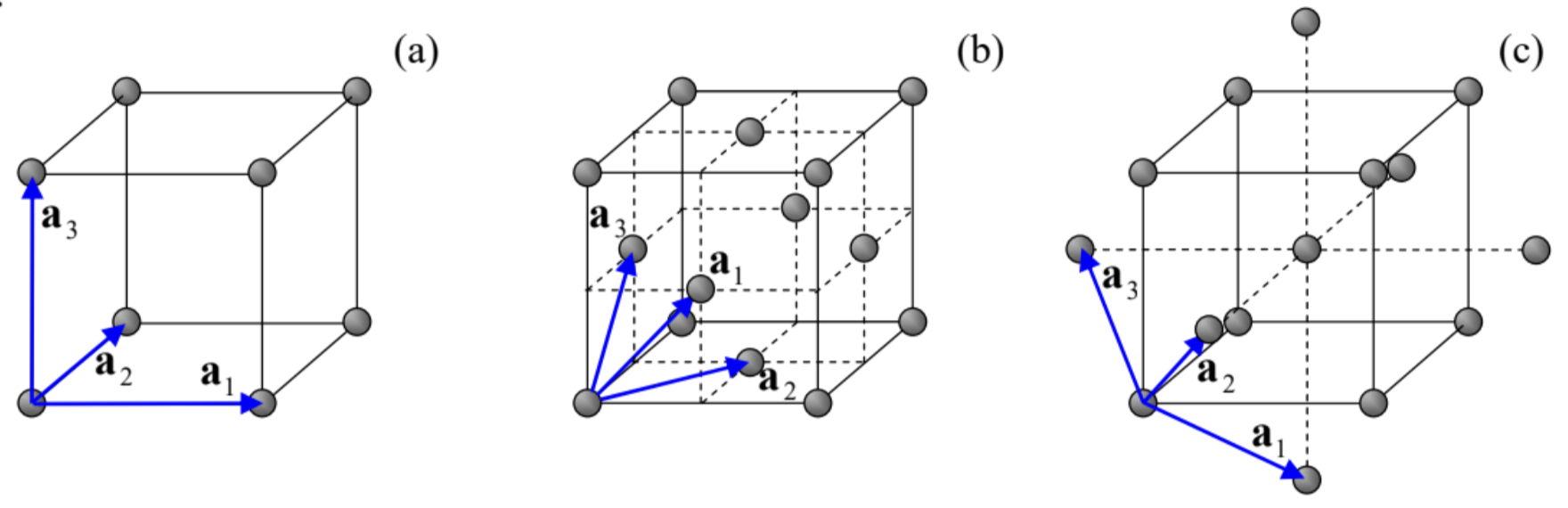
In Sec. 2.7, we have discussed the 1D band theory for potential profiles U(x) that obey the periodicity condition (2.192). For what follows, let us notice that the condition may be rewritten as U(x+X)=U(x), where X=τa, with τ being an arbitrary integer. One may say that the set of points X forms a periodic 1D lattice in the direct (r-) space. We have also seen that each Bloch state (i.e., each eigenstate of the Schrödinger equation for such periodic potential) is characterized by the quasimomentum ℏq, and its energy does not change if q is changed by a multiple of 2π/a. Hence if we form, in the reciprocal (q-) space, a 1D lattice of points Q=lb, with b≡2π/a and integer l, any pair of points from these two mutually reciprocal lattices satisfies the following rule: exp{iQX}=exp{il2πaτa}≡e2πiτl=1. In this form, the results of Sec. 2.7 may be readily extended to d-dimensional periodic potentials whose translational symmetry obeys the following natural generalization of Eq. (103): U(r+R)=U(r), where the points R, which may be numbered by d integers τj, form the so-called Bravais lattice: 43 R=d∑j=1τjaj, with d primitive vectors aj. The simplest example of a 3D Bravais lattice is given by the simple cubic lattice (Fig. 11a), which may be described by a system of mutually perpendicular primitive vectors aj of equal length. However, not in any lattice these vectors are perpendicular; for example, Figs. 11 b and 11c show possible sets of the primitive vectors describing, respectively, the face-centered cubic (fcc) lattice and the body-centered cubic (bcc) lattice. In 3D, the science of crystallography, based on group theory, distinguishes, by their symmetry properties, 14 Bravais lattices grouped into 7 different lattice systems. 44
Note, however, not all highly symmetric sets of points form Bravais lattices. As probably the most striking example, the nodes of a very simple 2D honeycomb lattice (Fig.12a)45 cannot be described by a Bravais lattice - while those of the 2D hexagonal lattice shown in Fig. 12b, can. The most prominent 3D case of such a lattice is the diamond structure (Fig. 12c), which describes, in particular, silicon crystals. 46 In cases like these, the band theory is much facilitated by the fact that the Bravais lattices using some point groups (called primitive unit cells) may describe these systems. 47 For example, Fig. 12a shows a possible choice of the primitive vectors for the honeycomb lattice, with the primitive unit cell formed by any two adjacent points of the original lattice (say, within the dashed ovals on that panel). Similarly, the diamond lattice may be described as an fcc Bravais lattice with a two-point primitive unit cell - see Fig. 12c.
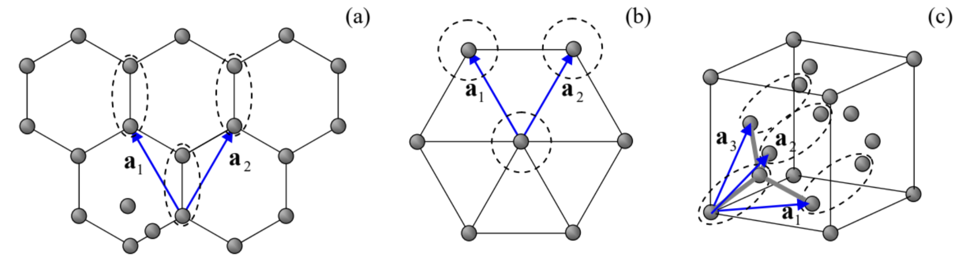 Fig. 3.12. Two important periodic structures that require two-point primitive cells for their Bravais lattice representation: (a) 2D honeycomb lattice and (c) 3D diamond lattice, and their primitive vectors. For contrast, panel (b) shows the 2D hexagonal structure which forms a Bravais lattice with a single-point primitive cell
Now we are ready for the following generalization of the 1D Bloch theorem, given by Eqs. (2.193) and (2.210), to higher dimensions: any eigenfunction of the Schrödinger equation describing particle’s motion in the spatially-unlimited periodic potential (105) may be represented either as
3D Bloch theorem or as ψ(r)=u(r)eiq⋅r, with u(r+R)=u(r)
where the quasimomentum ℏq is again a constant of motion, but now it is a vector. The key notion of the band theory in d dimensions is the reciprocal lattice in the wave-vector (q) space, formed as Q=d∑j=1ljbj, with integer lj, and vectors bj selected in such a way that the following natural generalization of Eq. (104) is valid for any pair of points of the direct and reciprocal lattices: eiQ⋅R=1. One way to describe the physical sense of the lattice Q is to say that according to Eqs. (80) and/or (86), it gives the set of the vectors q≡k−ki for that the interference of the waves scattered by all Bravais lattice points is constructive, and hence strongly enhanced. 48 Another way to look at the reciprocal lattice follows from the first formulation of the Bloch theorem, given by Eq. (107): if we add to the quasimomentum q of a particle any vector Q of the reciprocal lattice, the wavefunction does not change. This means, in particular, that all information about the system’s eigenfunctions is contained in just one elementary cell of the reciprocal space q. Its most frequent choice, called the 1St Brillouin zone, is the set of all points q that are closer to the origin than to any other point of the lattice Q. (Evidently, the 1st Brillouin zone in one dimension, discussed in Sec. 2.7, falls under this definition - see, e.g., Figs. 2.26 and 2.28.)
It is easy to see that the primitive vectors bj of the reciprocal lattice may be constructed as b1=2πa2×a3a1⋅(a2×a3),b2=2πa3×a1a1⋅(a2×a3),b3=2πa1×a2a1⋅(a2×a3). Indeed, from the "operand rotation rule" of the vector algebra 49 it is evident that aj⋅bj′=2πδjj ’. Hence, with the account of Eq. (109), the exponent on the left-hand side of Eq. (110) is reduced to eiQ⋅R=exp{2πi(l1τ1+l2τ2+l3τ3)}. Since all lj and all τj are integers, the expression in the parentheses is also an integer, so that the exponent indeed equals 1 , thus satisfying the definition of the reciprocal lattice given by Eq. (110).
As the simplest example, let us return to the simple cubic lattice of a period a (Fig. 11a), oriented in space so that a1=anx,a2=any,a3=anz, According to Eq. (111), its reciprocal lattice is also cubic: Q=2πa(lxnx+lyny+lznz), so that the 1st Brillouin zone is a cube with the side b=2π/a.
Almost equally simple calculations show that the reciprocal lattice of fcc is bec, and vice versa. Figure 13 shows the resulting 1st Brillouin zone of the fcc lattice.
The notion of the reciprocal lattice makes the multi-dimensional band theory not much more complex than that in 1D, especially for numerical calculations, at least for the single-point Bravais lattices. Indeed, repeating all the steps that have led us to Eq. (2.218), but now with a d-dimensional Fourier expansion of the functions U(r) and u(r), we readily get its generalization: ∑1′≠1U1′−1u1′=(E−E1)u1, where I is now a d-dimensional vector of integer indices lj. The summation in Eq. (115) should be carried over all essential components of this vector (i.e. over all relevant nodes of the reciprocal lattice), so that writing a corresponding computer code requires a bit more care than in 1D. However, this is just a homogeneous system of linear equations, and numerous routines of finding its eigenvalues E are readily available from both public sources and commercial software packages.
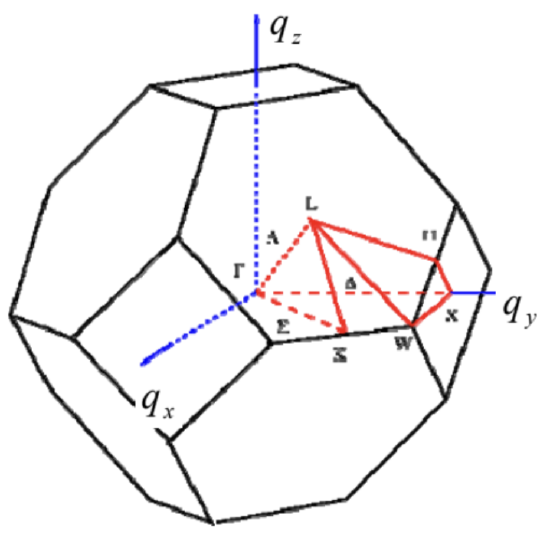
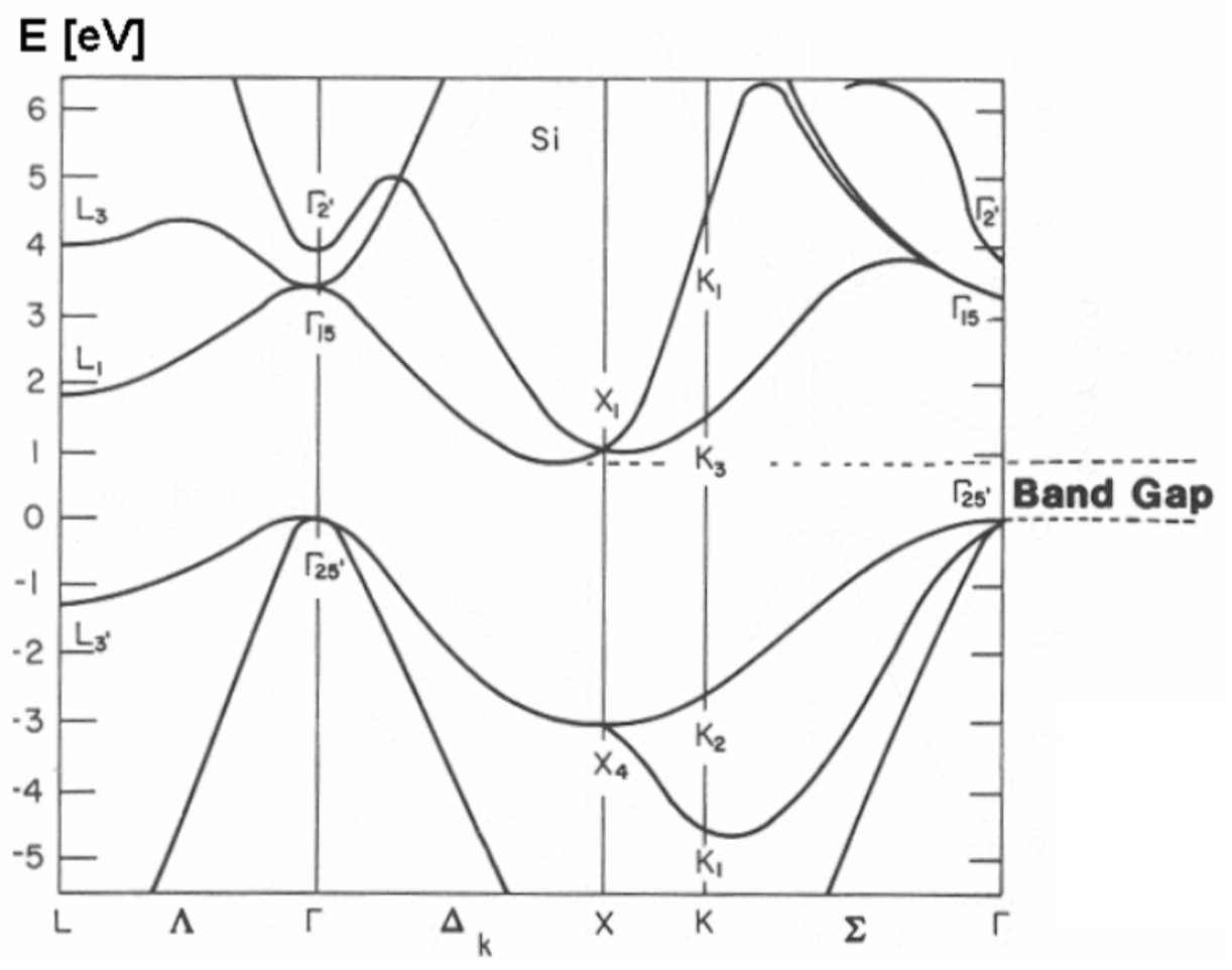
What is indeed more complex than in 1D is representation (and hence comprehension :-), of the calculated results and experimental data. Typically, the representation is limited to plotting the Bloch state eigenenergy as a function of components of the vector q along certain special directions the reciprocal space of quasimomentum (see, e.g., the red lines in Fig. 13), typically on a single panel. Fig. 14 shows perhaps the most famous (and certainly the most practically important) of such plots, the band structure of electrons in crystalline silicon. The dashed horizontal lines mark the so-called indirect gap of the width ∼1.12eV between the "valence" (nominally occupied) and the next "conduction" (nominally unoccupied) energy bands.
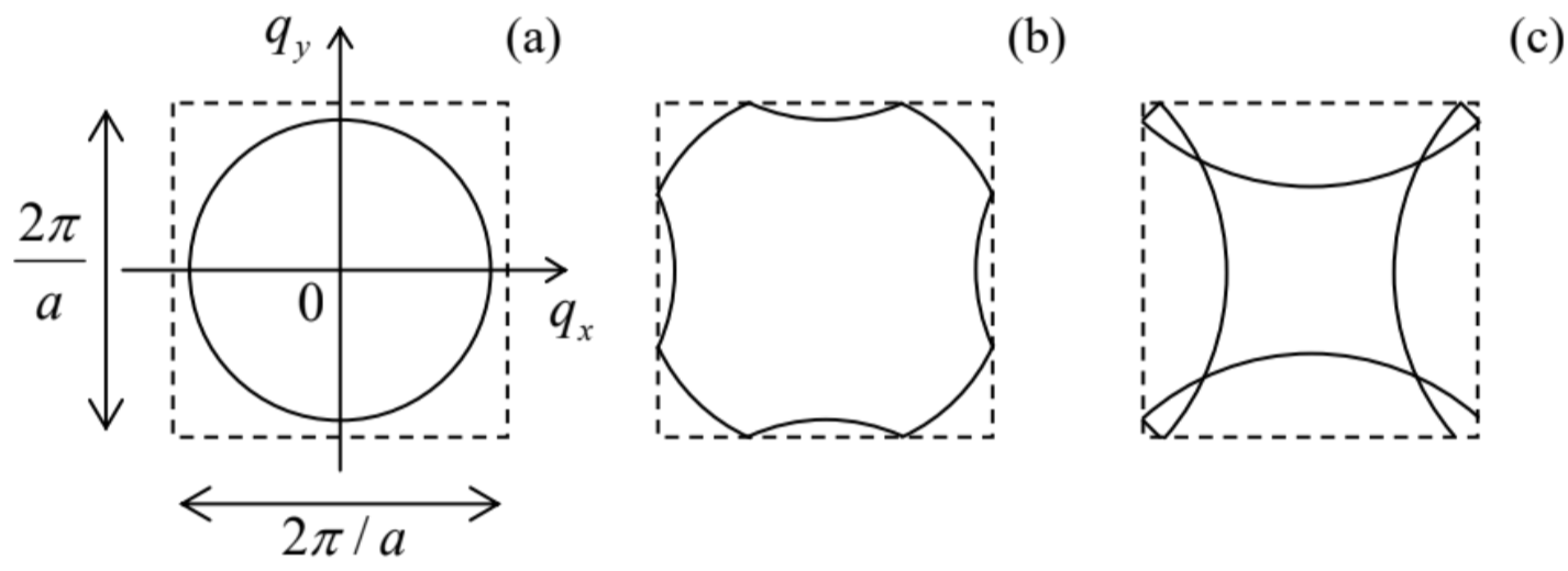
In order to understand the reason for such complexity, let us see how would we start to calculate such a picture in the weak-potential approximation, for the simplest case of a 2D square lattice − which is a subset of the cubic lattice (106), with τ3=0. Its 1st Brillouin zone is of course also a square, of the area (2π/a)2− see the dashed lines in Fig. 15. Let us draw the lines of the constant energy of a free particle (U=0) in this zone. Repeating the arguments of Sec. 2.7 (see especially Fig. 2.28 and its discussion), we may conclude that Eq. (2.216) should be now generalized as follows, E=ℏ2k22m=ℏ22m[(qx−2πlxa)2+(qy−2πlya)2] with all possible integers lx and ly. Considering this result only within the 1st Brillouin zone, we see that as the particle’s energy E grows, the lines of equal energy, for the lowest energy band, evolve as shown in Fig. 15. Just like in 1D, the weak-potential effects are only important at the Brillouin zone boundaries, and may be crudely considered as the appearance of narrow energy gaps, but one can see that the band structure in q-space is complex enough even without these effects - and becomes even more involved at higher E.
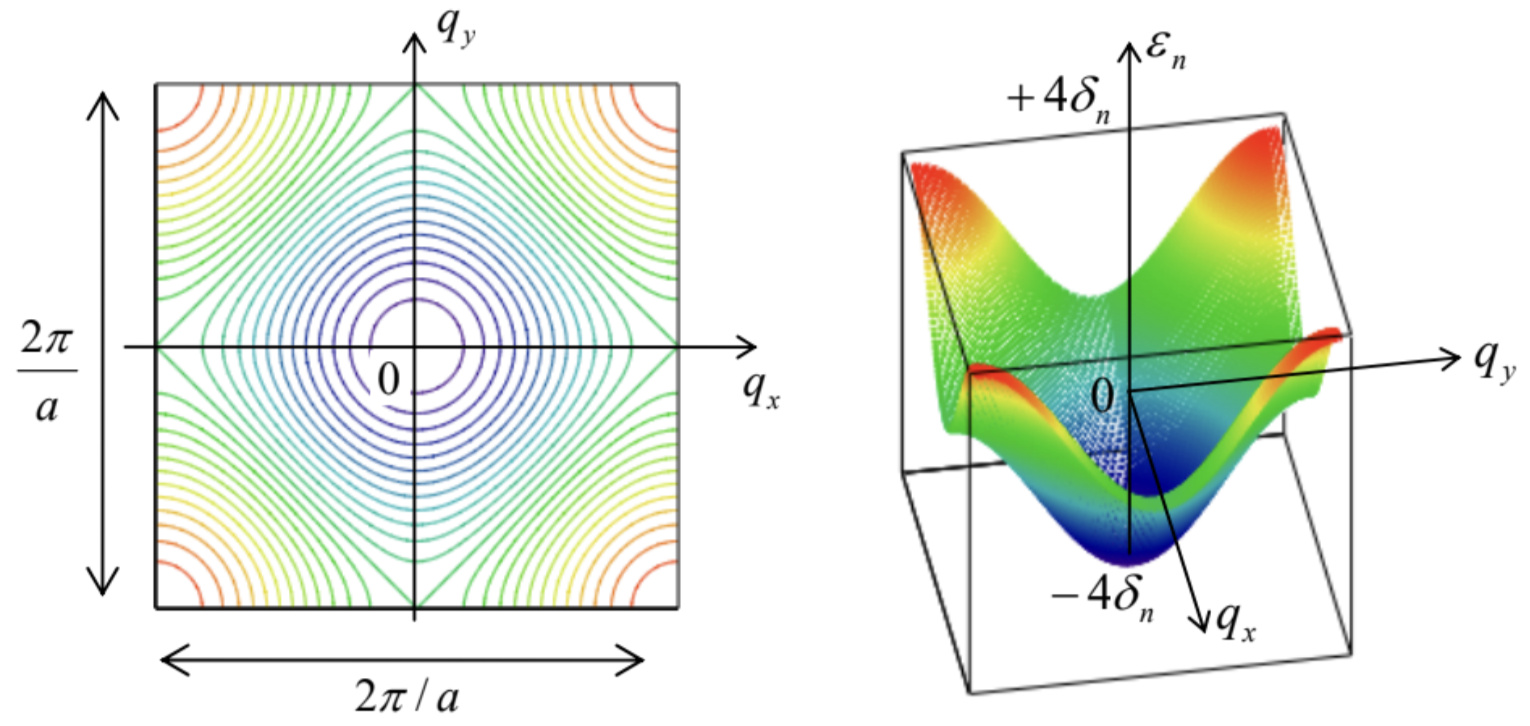
The tight-binding approximation is usually easier to follow. For example, for the same square 2D lattice, we may repeat the arguments that have led us to Eq. (2.203), to write 50 iℏ˙a0,0=−δn(a−1,0+a+1,0+a0,+1+a0,−1), where the indices correspond to the deviations of the integers τx and τy from an arbitrarily selected minimum of the potential energy - and hence of the wavefunction’s "hump", quasi-localized at this minimum. Now, looking for the stationary solution of these equations, that would obey the Bloch theorem (107), instead of Eq. (2.206) we get E=En+εn=En−δn(eiqxa+e−iqxa+eiqya+e−iqya)≡En−2δn(cosqxa+cosqya). Figure 16 shows this result, within the 1st Brillouin zone, in two forms: as color-coded lines of equal energy, and as a 3D plot (also enhanced by color). It is evident that the plots of this function along different lines on the q-plane, for example along one of the axes (say, qx ) and along a diagonal of the 1st Brillouin zone (say, with qx=qy ) give different curves E(q), qualitatively similar to those of silicon (Fig.
14). However, the latter structure is further complicated by the fact that the primitive cell of its Bravais lattice contains 2 atoms - see Fig. 12c and its discussion. In this case, even the tight-binding picture becomes more complex. Indeed, even if the atoms at different positions of the primitive unit cell are similar (as they are, for example, in both graphene and silicon), and hence the potential wells near those points and the corresponding local wavefunctions u(r) are similar as well, the Bloch theorem (which only pertains to Bravais lattices!) does not forbid them to have different complex probability amplitudes a(t) whose time evolution should be described by a specific differential equation.
As the simplest example, to describe the honeycomb lattice shown in Fig. 12a, we have to prescribe different probability amplitudes to the "top" and "bottom" points of its primitive cell - say, α and β, correspondingly. Since each of these points is surrounded (and hence weakly interacts) with three neighbors of the opposite type, instead of Eq. (117) we have to write two equations: iℏ˙α=−δn3∑j=1βj,iℏ˙β=−δn3∑j′=1αj′, where each summation is over three next-neighbor points. (In these two sums, I am using different summation indices just to emphasize that these directions are different for the "top" and "bottom" points of the primitive cell - see Fig. 12a.) Now using the Bloch theorem (107) in the form similar to Eq. (2.205), we get two coupled systems of linear algebraic equations: (E−En)α=−δnβ3∑j=1eiq⋅rj,(E−En)β=−δnα3∑j′=1eiq⋅r′j′, where rj and r′j′ are the next-neighbor positions, as seen from the top and bottom points, respectively. Writing the condition of consistency of this system of homogeneous linear equations, we get two equal and opposite values for energy correction for each value of q : E±=En±δnΣ1/2, where Σ≡3∑j,j′=1eiq⋅(rj+r′j′). According to Eq. (120), these two energy bands correspond to the phase shifts (on the top of the regular Bloch shift q⋅Δr) of either 0 or π between the adjacent quasi-localized wavefunctions u(r). The most interesting corollary of such energy symmetry, augmented by the honeycomb lattice’s symmetry, is that for certain values qD of the vector q (that turn out to be in each of six corners of the honeycomb-shaped 1st Brillouin zone), the double sum Σ vanishes, i.e. the two band surfaces E±(q) touch each other. As a result, in the vicinities of these so-called Dirac points, 51 the dispersion relation is linear: E±|q≈qD≈En±ℏvn|˜q|, where ˜q≡q−qD, with vn∝δn being a constant with the dimension of velocity - for graphene, close to 106 m/s. Such a linear dispersion relation ensures several interesting transport properties of graphene, in particular of the quantum Hall effect in it - as was already mentioned in Sec. 2. For their more detailed discussion, I have to refer the reader to special literature. 52
43 Named after Auguste Bravais, the crystallographer who introduced this notion in 1850 .
44 A very clear, well-illustrated introduction to the Bravais lattices is given in Chapters 4 and 7 of the famous textbook by N. Ashcroft and N. Mermin, Solid State Physics, Saunders College, 1976.
45 This structure describes, for example, the now-famous graphene: isolated monolayer sheets of carbon atoms arranged in a honeycomb lattice with an interatomic distance of 0.142 nm.
46 This diamond structure may be best understood as an overlap of two fcc lattices of side a, mutually shifted by the vector {1,1,1}×a/4, so that the distances between each point of the combined lattice and its 4 nearest neighbors (see the solid gray lines in Fig. 12c) are all equal.
47 A harder case is presented by so-called quasicrystals (whose idea may be traced down to medieval Islamic tilings, but was discovered in natural crystals, by D. Shechtman et al., only in 1984), which obey a high (say, the 5 -fold) rotational symmetry, but cannot be described by a Bravais lattice with any finite primitive unit cell. For a popular review of quasicrystals see, for example, P. Stephens and A. Goldman, Sci. Amer. 264, #4, 24 (1991).
48 This is why the notion of the Q-lattice is also the main starting point of X-ray diffraction studies of crystals. Indeed, it allows rewriting the well-known Bragg condition for diffraction peaks in an extremely simple form: k= ki+Q, where ki and k are the wave vectors of the, respectively, incident and diffracted waves − see, e.g., EM Sec. 8.4 (where it was more convenient for me to use the notation k0 for ki ).
49 See, e.g., MA Eq. (7.6).
50 Actually, using the same values of δn in both directions (x and y) implies some sort of symmetry of the quasilocalized states. For example, the s-states of axially-symmetric potentials (see the next section) always have such symmetry.
51 This term is based on a (rather indirect) analogy with the Dirac theory of relativistic quantum mechanics, to be discussed in Chapter 9 below.
52 See, e.g., the reviews by A. Castro Neto et al., Rev. Mod. Phys. 81,109 (2009) and by X. Lu et al., Appl. Phys. Rev. 4,021306 (2017). Note that the transport properties of graphene are determined by coupling of 2p-state electrons of its carbon atoms (see Secs. 6 and 7 below), whose wavefunctions are proportional to exp {±iφ} rather than are axially-symmetric as implied by Eqs. (120). However, due to the lattice symmetry, this fact does not affect the above dispersion relation E(q).